 生信宝典
生信宝典


写在前面
ggCLusterNet开发已历时两年,去年开始公开使用,不到一年的时间,谷歌上引用过ggClusterNet的文章数量已达23次。如今文章出来了,大家可以通过谷歌学术搜索ggClusterNet或文章主页(https://onlinelibrary.wiley.com/doi/full/10.1002/imt2.32)优雅地引用了。
全文翻译和视频简介见:《iMeta | 南农沈其荣团队发布微生物网络分析和可视化R包ggClusterNet》
欢迎大家扫描助手微信,备注R包,即可加入ggClusterNet用户交流群。

现发布包的使用教程,目录如下:

ggClusterNet:包含多种基于模块可视化布局算法的微生物网络挖掘R包
ggClusterNet: An R package for microbiome network analysis and modularity‐based multiple network layouts
作者:文涛#(wechat: nanjingxuezi),谢鹏昊#,杨胜蝶,牛国庆,刘潇予,丁哲旭,薛超,刘永鑫,沈其荣,袁军(junyuan@njau.edu.cn)
网络分析逐渐被生态学家们重视并持续应用于生态学领域,开发更为强大和方便的网络分析工具十分必要。因此,我们开发了名为ggClusterNet的R包,用于更加容易的进行网络数据分析挖掘和可视化。在ggClusterNet包中设计了数十种网络布局算法用于更好的展示微生物网络模块化信息(randomClusterG, PolygonClus-terG, PolygonRrClusterG, ArtifCluster, randSNEClusterG, PolygonModsquar-eG, PolyRdmNotdCirG, model_Gephi.2, model_igraph, model_maptree)。为了方便研究者使用,设计了多种微生物网络数据挖掘功能,例如相关性计算corMicor(),网络属性计算net_properties(),节点属性计算node_properties(),随机网络计算和比对random_Net_compate()。为了更加快捷挖掘网络,进一步将这些功能封装整合成两个函数network.2() 和 corBionetwork(),分别用于微生物网络数据挖掘和跨域网络数据挖掘。目前,ggClusterNet在GitHub: https://github.com/taowenmicro/ggClusterNet/ ,Gitee(https://gitee.com/wentaomicro/ggClusterNet)上开放使用。完整的说明和示例在wiki页面可以阅读。
ggClusterNet用于挖掘微生物网络和跨域网络,同时提供数十种基于模块化展示的网络布局算法。适应微生物组网络挖掘。
环境配置
R语言和Rstudio安装
R语言和Rstudio都是跨平台软件,从官方网站下载安装包进行安装:
R语言官方下载地址:https://www.r-project.org/
Rstudio官方下载地址:https://www.rstudio.com/products/rstudio/download/#download
测试代码和数据下载:在iMeta、宏基因组公众号后台回复“ggclusternet”
R包安装
方法1. Windows下批量下载R包解压安装
ggClusterNet依赖了十余个R包,如果安装存在困难,可以直接下载我编译好的安装包,这里还有一些其他R包,基本上都是用于组学分析等生物信息方面的分析。供win用户使用。
R 4.2系列的R包 321.56M 链接:https://pan.baidu.com/s/1xc-Eyz3GhJtZ6LaPOGhQWA?pwd=0315
备用链接含作者常用R包 2.08G接:https://pan.baidu.com/s/1pbumFhF-EC2atQTB0wuiMw?pwd=udf5 提取码:udf5
更新版获取方式,在iMeta、宏基因组公众号后台回复“ggclusternet”
使用方式为:下载后解压缩其中的所有目录到R语言安装路径中的4.2或library中,具体位置可执行 .libPaths() 查看。
> .libPaths()
[1] "C:/Users/yongxinliu/AppData/Local/R/win-library/4.2"
[2] "C:/Program Files/R/R-4.2.0/library"
最好复制到第一个用户目录中,为额外安装R包位置。第二个为系统目录,为软件自带R包位置。
方法2. 代码安装
# 基于CRAN安装R包
p_list = c("ggplot2", "BiocManager", "devtools", "igraph", "network", "sna", "tidyverse","tidyfst","ggnewscale")
for(p in p_list){if (!requireNamespace(p)){install.packages(p)}
    library(p, character.only = TRUE, quietly = TRUE, warn.conflicts = FALSE)}

# 基于Bioconductor安装R包
p_list = c("phyloseq", "WGCNA")
for(p in p_list){if (!requireNamespace(p, quietly = TRUE)){BiocManager::install(p)}}

# 基于github安装,检测没有则安装
library(devtools)
if (!requireNamespace("ggClusterNet", quietly = TRUE))
remotes::install_github("taowenmicro/ggClusterNet")导入R包
#--导入所需R包#-------
library(phyloseq)
library(igraph)
library(network)
library(sna)
library(tidyverse)
library(ggClusterNet)
数据
输入方式一
直接输入phyloseq格式的数据。
#-----导入数据#-------
data(ps)
输入方式二
可以从https://github.com/taowenmicro/R-_function下载数据,构造phylsoeq文件。自己的数据也按照网址示例数据进行准备。虽然phylsoeq对象不易用常规手段处理,但是组学数据由于数据量比较大,数据注释内容多样化,所以往往使用诸如phyloseq这类对象进行处理,并简化数据处理过程。ggClusterNet同样使用了phyloseq对象作为微生物网络的分析。
phyloseq对象构建过程如下,网络分析主要用到otu表格,后续pipeline流程可能用到分组文件metadata,如果按照分类水平山色或者区分模块则需要taxonomy。这几个部分并不是都必须加入phyloseq对象中,可以用到哪个加哪个。
library(phyloseq)
library(ggClusterNet)
library(tidyverse)
library(Biostrings)

metadata = read.delim("./metadata.tsv",row.names = 1)
otutab = read.delim("./otutab.txt", row.names=1)
taxonomy = read.table("./taxonomy.txt", row.names=1)
# tree  = read_tree("./otus.tree")
# rep = readDNAStringSet("./otus.fa")

ps = phyloseq(sample_data(metadata),
              otu_table(as.matrix(otutab), taxa_are_rows=TRUE),
              tax_table(as.matrix(taxonomy))#,
              # phy_tree(tree),
              # refseq(rep)
              )
或者直接从网站读取,但是由于github在国外,所以容易失败
metadata = read.delim("https://raw.githubusercontent.com/taowenmicro/R-_function/main/metadata.tsv",row.names = 1)
otutab = read.delim("https://raw.githubusercontent.com/taowenmicro/R-_function/main/otutab.txt", row.names=1)
taxonomy = read.table("https://raw.githubusercontent.com/taowenmicro/R-_function/main/taxonomy.txt", row.names=1)
# tree  = read_tree("https://raw.githubusercontent.com/taowenmicro/R-_function/main/otus.tree")
# rep = readDNAStringSet("https://raw.githubusercontent.com/taowenmicro/R-_function/main/otus.fa")

ps = phyloseq(sample_data(metadata),
              otu_table(as.matrix(otutab), taxa_are_rows=TRUE),
              tax_table(as.matrix(taxonomy))#,
              # phy_tree(tree),
              # refseq(rep)
              )
使用ggCLusterNet进行网络分析的过程
corMicro函数用于计算网络相关
按照丰度过滤微生物表格,并却计算相关矩阵,按照指定的阈值挑选矩阵中展示的数值。调用了psych包中的corr.test函数,使用三种相关方法。
N参数提取丰度最高的150个OTU;
method.scale参数确定微生物组数据的标准化方式,这里我们选用TMM方法标准化微生物数据。
#-提取丰度最高的指定数量的otu进行构建网络

#----------计算相关#----
result = corMicro (ps = ps,
                   N = 150,
                   method.scale = "TMM",
                   r.threshold=0.8,
                   p.threshold=0.05,
                   method = "spearman"


                   )

#--提取相关矩阵
cor = result[[1]]
head(cor)

#-网络中包含的OTU的phyloseq文件提取
ps_net = result[[3]]

#-导出otu表格
otu_table = ps_net %>%
  vegan_otu() %>%
  t() %>%
  as.data.frame()
制作分组,我们模拟五个分组
ggClusterNet中提供了多种优秀的网络可视化布局算法:
PolygonClusterG:环状模块,环状布局
PolygonRrClusterG:环状模块,模块半径正比于节点数量,环状布局
randomClusterG:随机布局,环状模块
ArtifCluster:环状模块,人工布局
randSNEClusterG:sna包中的布局按照模块布局
PolygonModsquareG 环状布局,顺序行列排布
PolygonRdmNodeCir 实心圈布局,环状布局,控制半径
model_Gephi.2:模仿Gephi布局
model_igraph:模仿igraph布局
model_maptree:按照maptree算法布局模块
model_maptree2:内聚算法改进离散点排布
model_filled_circle 实心圆布局,基于分组信息
等···········
这是网络布局的基础,无论是什么聚类布局,都需要制作一个分组文件,这个文件有两列,一列是节点,一列是分组信息,这个分组信息名称为:group。这个文件信息就是用于对节点进行分组,然后按照分组对节点归类,使用包中可视化函数计算节点位置。
注意分组文件的格式,分为两列,第一列是网络中包含的OTU的名字,第二列是分组信息,同样的分组标记同样的字符。
#--人工构造分组信息:将网络中全部OTU分为五个部分,等分
netClu = data.frame(ID = row.names(otu_table),group =rep(1:5,length(row.names(otu_table)))[1:length(row.names(otu_table))] )
netClu$group = as.factor(netClu$group)
head(netClu)
PolygonClusterG 根据分组,计算布局位置坐标
不同的模块按照分组聚集成不同的圆,并且圆形的大小一样。如果一个分组只有一个点,则这个点坐落在圆心位置。
#--------计算布局#---------
result2 = PolygonClusterG (cor = cor,nodeGroup =netClu  )
node = result2[[1]]
head(node)
nodeadd 节点注释的:用otu表格和分组文件进行注释
nodeadd函数只是提供了简单的用注释函数,用户可以自己在node的表格后面添加各种注释信息。
tax_table = ps_net %>%
  vegan_tax() %>%
  as.data.frame()
#---node节点注释#-----------
nodes = nodeadd(plotcord =node,otu_table = otu_table,tax_table = tax_table)
head(nodes)
计算边
#-----计算边#--------
edge = edgeBuild(cor = cor,node = node)
head(edge)
出图
p <- ggplot() + geom_segment(aes(x = X1, y = Y1, xend = X2, yend = Y2,color = as.factor(cor)),
                                data = edge, size = 0.5) +
  geom_point(aes(X1, X2,fill = Phylum,size = mean),pch = 21, data = nodes) +
  scale_colour_brewer(palette = "Set1") +
  scale_x_continuous(breaks = NULL) + scale_y_continuous(breaks = NULL) +
  theme(panel.background = element_blank()) +
  theme(axis.title.x = element_blank(), axis.title.y = element_blank()) +
  theme(legend.background = element_rect(colour = NA)) +
  theme(panel.background = element_rect(fill = "white",  colour = NA)) +
  theme(panel.grid.minor = element_blank(), panel.grid.major = element_blank())
p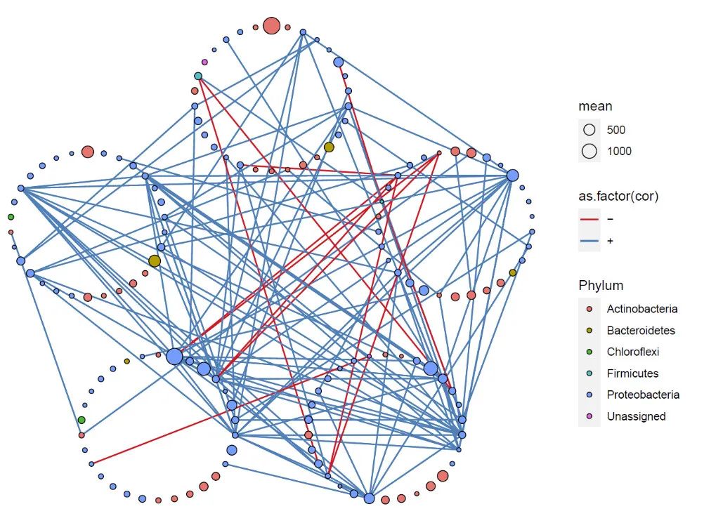
模拟不同的分组—可视化
模拟不同分组效果展示:1个分组
这是网络布局的基础,无论是什么聚类布局,都需要制作一个分组文件,这个文件有两列,一列是节点,一列是分组信息,这个分组信息名称必须设定为:group。
netClu = data.frame(ID = row.names(tax_table),group =rep(1,length(row.names(tax_table)))[1:length(row.names(tax_table))] )
netClu$group = as.factor(netClu$group)
result2 = PolygonClusterG (cor = cor,nodeGroup =netClu )
node = result2[[1]]
# ---node节点注释#-----------
nodes = nodeadd(plotcord =node,otu_table = otu_table,tax_table = tax_table)

#-----计算边#--------
edge = edgeBuild(cor = cor,node = node)

### 出图
pnet <- ggplot() + geom_segment(aes(x = X1, y = Y1, xend = X2, yend = Y2,color = as.factor(cor)),
                                data = edge, size = 0.5) +
  geom_point(aes(X1, X2,fill = Phylum,size = mean),pch = 21, data = nodes) +
  scale_colour_brewer(palette = "Set1") +
  scale_x_continuous(breaks = NULL) + scale_y_continuous(breaks = NULL) +
  # labs( title = paste(layout,"network",sep = "_"))+
  # geom_text_repel(aes(X1, X2,label=Phylum),size=4, data = plotcord)+
  # discard default grid + titles in ggplot2
  theme(panel.background = element_blank()) +
  # theme(legend.position = "none") +
  theme(axis.title.x = element_blank(), axis.title.y = element_blank()) +
  theme(legend.background = element_rect(colour = NA)) +
  theme(panel.background = element_rect(fill = "white",  colour = NA)) +
  theme(panel.grid.minor = element_blank(), panel.grid.major = element_blank())
pnet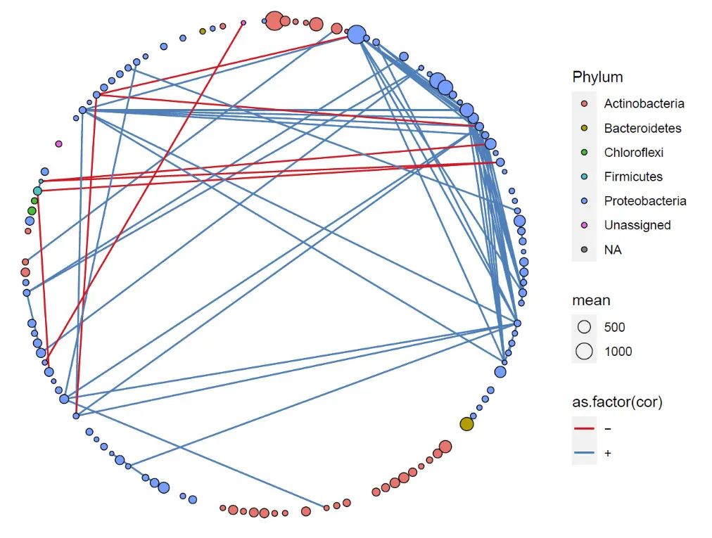
模拟不同的分组查看效果:8个分组
netClu = data.frame(ID = row.names(cor),group =rep(1:8,length(row.names(cor)))[1:length(row.names(cor))] )
netClu$group = as.factor(netClu$group)
result2 = PolygonClusterG (cor = cor,nodeGroup =netClu )
node = result2[[1]]
# ---node节点注释#-----------
nodes = nodeadd(plotcord =node,otu_table = otu_table,tax_table = tax_table)
#-----计算边#--------
edge = edgeBuild(cor = cor,node = node)
### 出图
pnet <- ggplot() + geom_segment(aes(x = X1, y = Y1, xend = X2, yend = Y2,color = as.factor(cor)),
                                data = edge, size = 0.5) +
  geom_point(aes(X1, X2,fill = Phylum,size = mean),pch = 21, data = nodes) +
  scale_colour_brewer(palette = "Set1") +
  scale_x_continuous(breaks = NULL) + scale_y_continuous(breaks = NULL) +
  # labs( title = paste(layout,"network",sep = "_"))+
  # geom_text_repel(aes(X1, X2,label=Phylum),size=4, data = plotcord)+
  # discard default grid + titles in ggplot2
  theme(panel.background = element_blank()) +
  # theme(legend.position = "none") +
  theme(axis.title.x = element_blank(), axis.title.y = element_blank()) +
  theme(legend.background = element_rect(colour = NA)) +
  theme(panel.background = element_rect(fill = "white",  colour = NA)) +
  theme(panel.grid.minor = element_blank(), panel.grid.major = element_blank())
pnet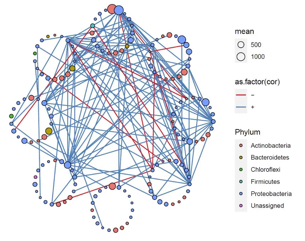
按照微生物分类不同设定分组
#----------计算相关#----
result = corMicro (ps = ps,
                   N = 200,
                   method.scale = "TMM",
                   r.threshold=0.8,
                   p.threshold=0.05,
                   method = "spearman"
                   )
#--提取相关矩阵
cor = result[[1]]
head(cor)
#-网络中包含的OTU的phyloseq文件提取
ps_net = result[[3]]
#-导出otu表格
otu_table = ps_net %>%
  vegan_otu() %>%
  t() %>%
  as.data.frame()
tax = ps_net %>% vegan_tax() %>%
  as.data.frame()
tax$filed = tax$Phylum
group2 <- data.frame(ID = row.names(tax),group = tax$Phylum)
group2$group  =as.factor(group2$group)
result2 = PolygonClusterG (cor = cor,nodeGroup =group2 )
node = result2[[1]]
# ---node节点注释#-----------
nodes = nodeadd(plotcord =node,otu_table = otu_table,tax_table = tax_table)
#-----计算边#--------
edge = edgeBuild(cor = cor,node = node)
### 出图
pnet <- ggplot() + geom_segment(aes(x = X1, y = Y1, xend = X2, yend = Y2,color = as.factor(cor)),
                                data = edge, size = 0.5) +
  geom_point(aes(X1, X2,fill = Phylum,size = mean),pch = 21, data = nodes) +
  scale_colour_brewer(palette = "Set1") +
  scale_x_continuous(breaks = NULL) + scale_y_continuous(breaks = NULL) +
  # labs( title = paste(layout,"network",sep = "_"))+
  # geom_text_repel(aes(X1, X2,label=Phylum),size=4, data = plotcord)+
  # discard default grid + titles in ggplot2
  theme(panel.background = element_blank()) +
  # theme(legend.position = "none") +
  theme(axis.title.x = element_blank(), axis.title.y = element_blank()) +
  theme(legend.background = element_rect(colour = NA)) +
  theme(panel.background = element_rect(fill = "white",  colour = NA)) +
  theme(panel.grid.minor = element_blank(), panel.grid.major = element_blank())
pnet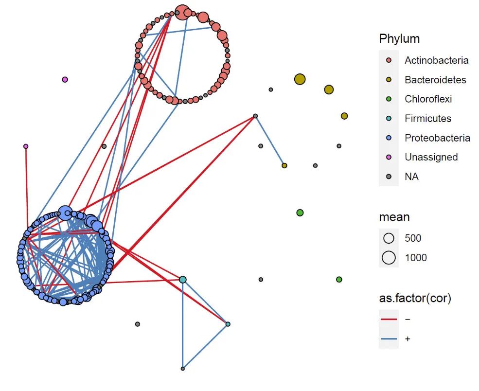
结果发现这些高丰度OTU大部分属于放线菌门和变形菌门,其他比较少。所以下面我们按照OTU数量的多少,对每个模块的大小进行重新调整。
result2 = PolygonRrClusterG (cor = cor,nodeGroup =group2 )
node = result2[[1]]
# ---node节点注释#-----------
nodes = nodeadd(plotcord =node,otu_table = otu_table,tax_table = tax_table)
#-----计算边#--------
edge = edgeBuild(cor = cor,node = node)
### 出图
pnet <- ggplot() + geom_segment(aes(x = X1, y = Y1, xend = X2, yend = Y2,color = as.factor(cor)),
                                data = edge, size = 0.5) +
  geom_point(aes(X1, X2,fill = Phylum,size = mean),pch = 21, data = nodes) +
  scale_colour_brewer(palette = "Set1") +
  scale_x_continuous(breaks = NULL) + scale_y_continuous(breaks = NULL) +
  # labs( title = paste(layout,"network",sep = "_"))+
  # geom_text_repel(aes(X1, X2,label=Phylum),size=4, data = plotcord)+
  # discard default grid + titles in ggplot2
  theme(panel.background = element_blank()) +
  # theme(legend.position = "none") +
  theme(axis.title.x = element_blank(), axis.title.y = element_blank()) +
  theme(legend.background = element_rect(colour = NA)) +
  theme(panel.background = element_rect(fill = "white",  colour = NA)) +
  theme(panel.grid.minor = element_blank(), panel.grid.major = element_blank())
pnet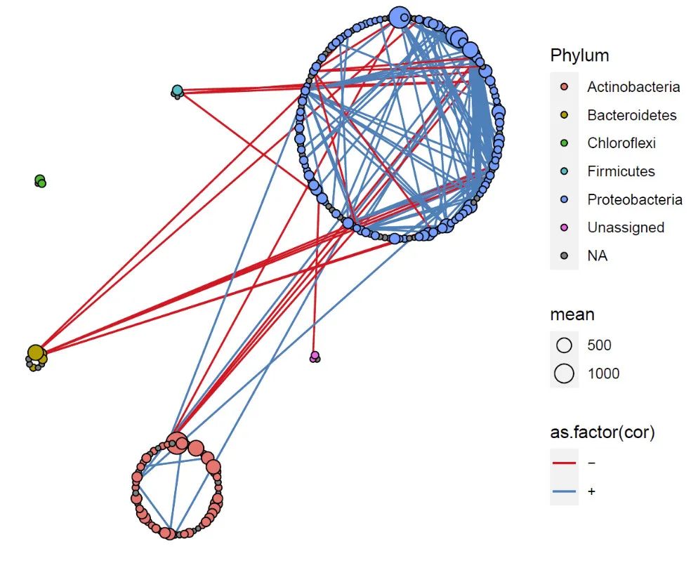
用实心点作为每个模块的布局方式1
set.seed(12)
#-实心圆2
result2 = model_filled_circle(cor = cor,
                              culxy =TRUE,
                              da = NULL,# 数据框,包含x,和y列
                              nodeGroup = group2,
                              mi.size = 1,# 最小圆圈的半径,越大半径越大
                              zoom = 0.3# 不同模块之间距离
                              )

# result2 = PolygonRrClusterG (cor = cor,nodeGroup =group2 )
node = result2[[1]]
# ---node节点注释#-----------
nodes = nodeadd(plotcord =node,otu_table = otu_table,tax_table = tax_table)
#-----计算边#--------
edge = edgeBuild(cor = cor,node = node)
### 出图
pnet <- ggplot() + geom_segment(aes(x = X1, y = Y1, xend = X2, yend = Y2,color = as.factor(cor)),
                                data = edge, size = 0.5) +
  geom_point(aes(X1, X2,fill = Phylum,size = mean),pch = 21, data = nodes) +
  scale_colour_brewer(palette = "Set1") +
  scale_x_continuous(breaks = NULL) + scale_y_continuous(breaks = NULL) +
  # labs( title = paste(layout,"network",sep = "_"))+
  # geom_text_repel(aes(X1, X2,label=Phylum),size=4, data = plotcord)+
  # discard default grid + titles in ggplot2
  theme(panel.background = element_blank()) +
  # theme(legend.position = "none") +
  theme(axis.title.x = element_blank(), axis.title.y = element_blank()) +
  theme(legend.background = element_rect(colour = NA)) +
  theme(panel.background = element_rect(fill = "white",  colour = NA)) +
  theme(panel.grid.minor = element_blank(), panel.grid.major = element_blank())
pnet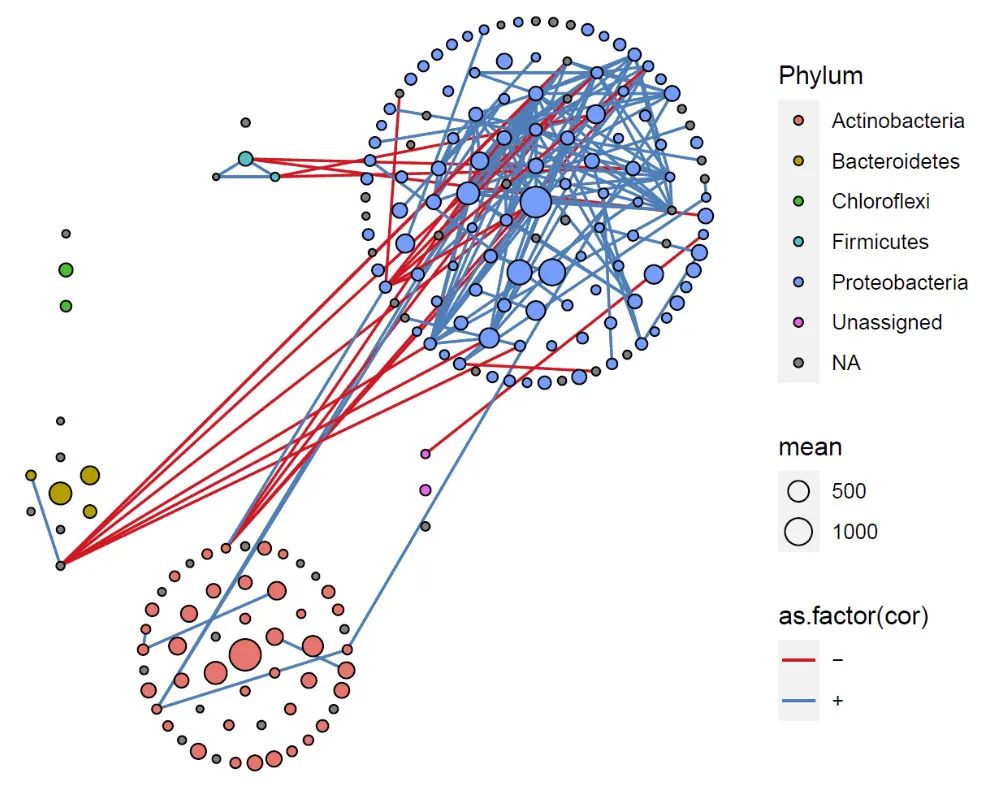
用实心点作为每个模块布局方式2
set.seed(12)
#-实心圆2
result2 = model_maptree_group(cor = cor,
                              nodeGroup = group2,
                              )

# result2 = PolygonRrClusterG (cor = cor,nodeGroup =group2 )
node = result2[[1]]
# ---node节点注释#-----------
nodes = nodeadd(plotcord =node,otu_table = otu_table,tax_table = tax_table)
#-----计算边#--------
edge = edgeBuild(cor = cor,node = node)
### 出图
pnet <- ggplot() + geom_segment(aes(x = X1, y = Y1, xend = X2, yend = Y2,color = as.factor(cor)),
                                data = edge, size = 0.5) +
  geom_point(aes(X1, X2,fill = Phylum,size = mean),pch = 21, data = nodes) +
  scale_colour_brewer(palette = "Set1") +
  scale_x_continuous(breaks = NULL) + scale_y_continuous(breaks = NULL) +
  # labs( title = paste(layout,"network",sep = "_"))+
  # geom_text_repel(aes(X1, X2,label=Phylum),size=4, data = plotcord)+
  # discard default grid + titles in ggplot2
  theme(panel.background = element_blank()) +
  # theme(legend.position = "none") +
  theme(axis.title.x = element_blank(), axis.title.y = element_blank()) +
  theme(legend.background = element_rect(colour = NA)) +
  theme(panel.background = element_rect(fill = "white",  colour = NA)) +
  theme(panel.grid.minor = element_blank(), panel.grid.major = element_blank())
pnet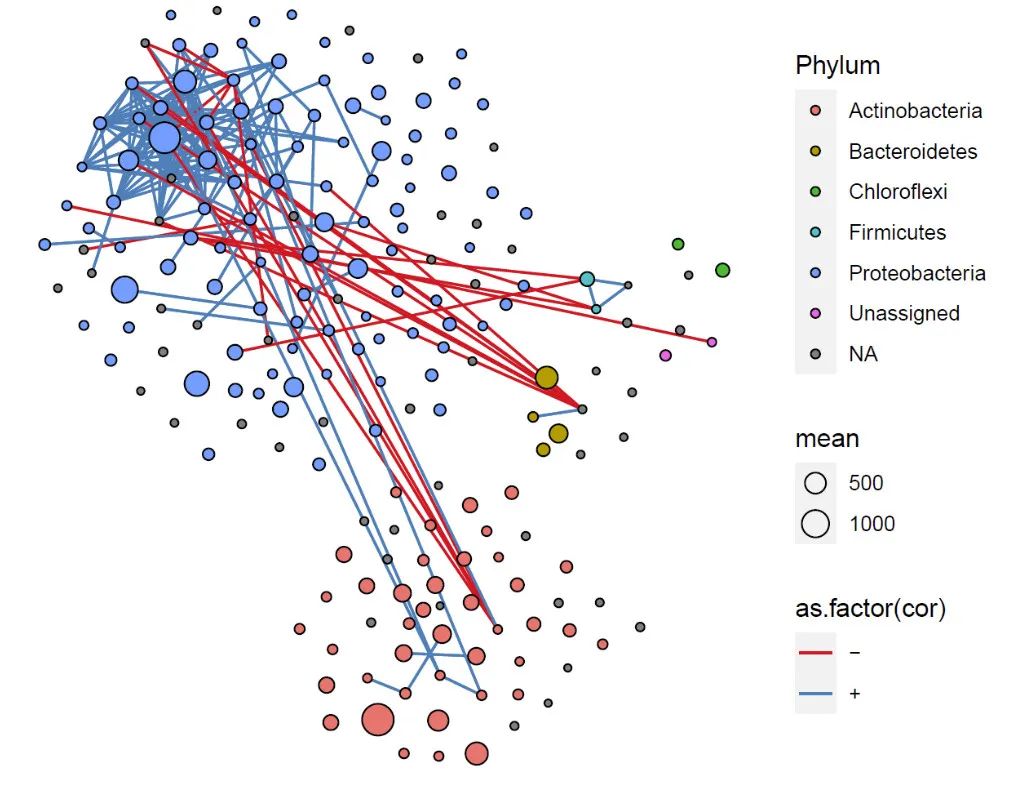
按照网络模块分析定义分组
netClu  = modulGroup( cor = cor,cut = NULL,method = "cluster_fast_greedy" )

result2 = model_maptree_group(cor = cor,
                              nodeGroup = group2,
                              )

# result2 = PolygonRrClusterG (cor = cor,nodeGroup =group2 )
node = result2[[1]]

# ---node节点注释#-----------
nodes = nodeadd(plotcord =node,otu_table = otu_table,tax_table = tax_table)
head(nodes)

nodes2 = nodes %>% inner_join(netClu,by = c("elements" = "ID"))
nodes2$group = paste("Model_",nodes2$group,sep = "")

#-----计算边#--------
edge = edgeBuild(cor = cor,node = node)

### 出图
pnet <- ggplot() + geom_segment(aes(x = X1, y = Y1, xend = X2, yend = Y2,color = as.factor(cor)),
                                data = edge, size = 0.5) +
  geom_point(aes(X1, X2,fill = group,size = mean),pch = 21, data = nodes2) +
  scale_colour_brewer(palette = "Set1") +
  scale_x_continuous(breaks = NULL) + scale_y_continuous(breaks = NULL) +
  # labs( title = paste(layout,"network",sep = "_"))+
  # geom_text_repel(aes(X1, X2,label=Phylum),size=4, data = plotcord)+
  # discard default grid + titles in ggplot2
  theme(panel.background = element_blank()) +
  # theme(legend.position = "none") +
  theme(axis.title.x = element_blank(), axis.title.y = element_blank()) +
  theme(legend.background = element_rect(colour = NA)) +
  theme(panel.background = element_rect(fill = "white",  colour = NA)) +
  theme(panel.grid.minor = element_blank(), panel.grid.major = element_blank())
pnet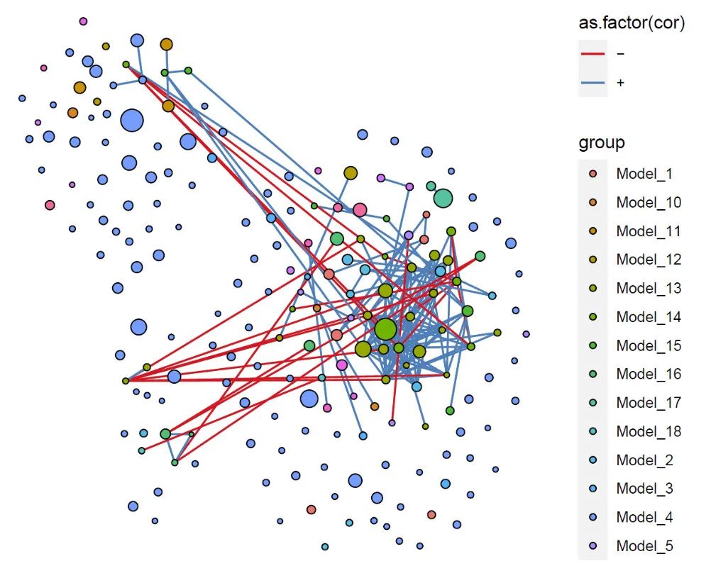
使用升级的model_maptree2:不在可以将每个模块独立区分,而是将模块聚拢,并在整体布局上将离散的点同这些模块一同绘制到同心圆内。
result2 = model_maptree2(cor = cor,
                              method = "cluster_fast_greedy"
                              )

# result2 = PolygonRrClusterG (cor = cor,nodeGroup =group2 )
node = result2[[1]]

# ---node节点注释#-----------
nodes = nodeadd(plotcord =node,otu_table = otu_table,tax_table = tax_table)
head(nodes)

nodes2 = nodes %>% inner_join(netClu,by = c("elements" = "ID"))
nodes2$group = paste("Model_",nodes2$group,sep = "")

#-----计算边#--------
edge = edgeBuild(cor = cor,node = node)

### 出图
pnet <- ggplot() + geom_segment(aes(x = X1, y = Y1, xend = X2, yend = Y2,color = as.factor(cor)),
                                data = edge, size = 0.5) +
  geom_point(aes(X1, X2,fill = group,size = mean),pch = 21, data = nodes2) +
  scale_colour_brewer(palette = "Set1") +
  scale_x_continuous(breaks = NULL) + scale_y_continuous(breaks = NULL) +
  # labs( title = paste(layout,"network",sep = "_"))+
  # geom_text_repel(aes(X1, X2,label=Phylum),size=4, data = plotcord)+
  # discard default grid + titles in ggplot2
  theme(panel.background = element_blank()) +
  # theme(legend.position = "none") +
  theme(axis.title.x = element_blank(), axis.title.y = element_blank()) +
  theme(legend.background = element_rect(colour = NA)) +
  theme(panel.background = element_rect(fill = "white",  colour = NA)) +
  theme(panel.grid.minor = element_blank(), panel.grid.major = element_blank())
pnet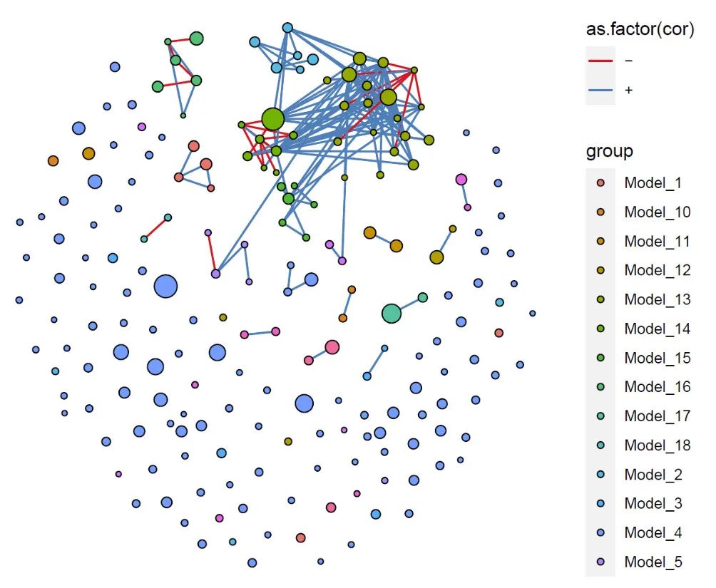
model_igraph布局
result = cor_Big_micro(ps = ps,
                   N = 1000,
                   r.threshold=0.6,
                   p.threshold=0.05,
                   method = "spearman"
                   )

#--提取相关矩阵
cor = result[[1]]
dim(cor)

result2 <- model_igraph(cor = cor,
                         method = "cluster_fast_greedy",
                         seed = 12
)
node = result2[[1]]
head(node)

dat = result2[[2]]
head(dat)
tem = data.frame(mod = dat$model,col = dat$color) %>%
  dplyr::distinct( mod, .keep_all = TRUE)
col = tem$col
names(col) = tem$mod

#---node节点注释#-----------
otu_table = as.data.frame(t(vegan_otu(ps)))
tax_table = as.data.frame(vegan_tax(ps))
nodes = nodeadd(plotcord =node,otu_table = otu_table,tax_table = tax_table)
head(nodes)
#-----计算边#--------
edge = edgeBuild(cor = cor,node = node)
colnames(edge)[8] = "cor"
head(edge)

tem2 = dat %>%
  dplyr::select(OTU,model,color) %>%
  dplyr::right_join(edge,by =c("OTU" = "OTU_1" ) ) %>%
  dplyr::rename(OTU_1 = OTU,model1 = model,color1 = color)
head(tem2)

tem3 = dat %>%
  dplyr::select(OTU,model,color) %>%
  dplyr::right_join(edge,by =c("OTU" = "OTU_2" ) ) %>%
  dplyr::rename(OTU_2 = OTU,model2 = model,color2 = color)
head(tem3)

tem4 = tem2 %>%inner_join(tem3)
head(tem4)

edge2 = tem4 %>% mutate(color = ifelse(model1 == model2,as.character(model1),"across"),
                        manual = ifelse(model1 == model2,as.character(color1),"#C1C1C1")
                        )
head(edge2)
col_edge = edge2 %>% dplyr::distinct(color, .keep_all = TRUE)  %>%
  select(color,manual)
col0 = col_edge$manual
names(col0) = col_edge$color

library(ggnewscale)

p1 <- ggplot() + geom_segment(aes(x = X1, y = Y1, xend = X2, yend = Y2,color = color),
                              data = edge2, size = 1) +
  scale_colour_manual(values = col0)

# ggsave("./cs1.pdf",p1,width = 16,height = 14)
p2 = p1 +
   new_scale_color() +
  geom_point(aes(X1, X2,color =model), data = dat,size = 4) +
  scale_colour_manual(values = col) +
  scale_x_continuous(breaks = NULL) + scale_y_continuous(breaks = NULL) +
  theme(panel.background = element_blank()) +
  theme(axis.title.x = element_blank(), axis.title.y = element_blank()) +
  theme(legend.background = element_rect(colour = NA)) +
  theme(panel.background = element_rect(fill = "white",  colour = NA)) +
  theme(panel.grid.minor = element_blank(), panel.grid.major = element_blank())
p2
# ggsave("./cs2.pdf",p2,width = 16,height = 14)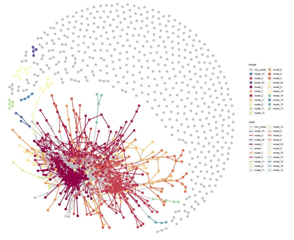
节点模块化计算和可视化
result4 = nodeEdge(cor = cor)
#提取变文件
edge = result4[[1]]
#--提取节点文件
node = result4[[2]]
igraph  = igraph::graph_from_data_frame(edge, directed = FALSE, vertices = node)
res = ZiPiPlot(igraph = igraph,method = "cluster_fast_greedy")
p <- res[[1]]
p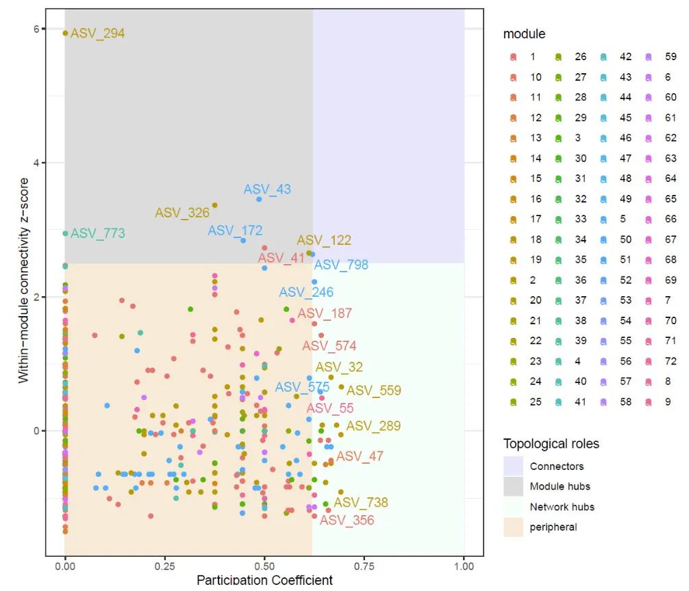
网络性质计算
22年6月升级后版本包括了16项网络属性,包括周集中老师21年NCC文章中全部属性
dat = net_properties(igraph)
head(dat)
# 升级后包含的网络属性更多
dat = net_properties.2(igraph,n.hub = T)
head(dat,n = 16)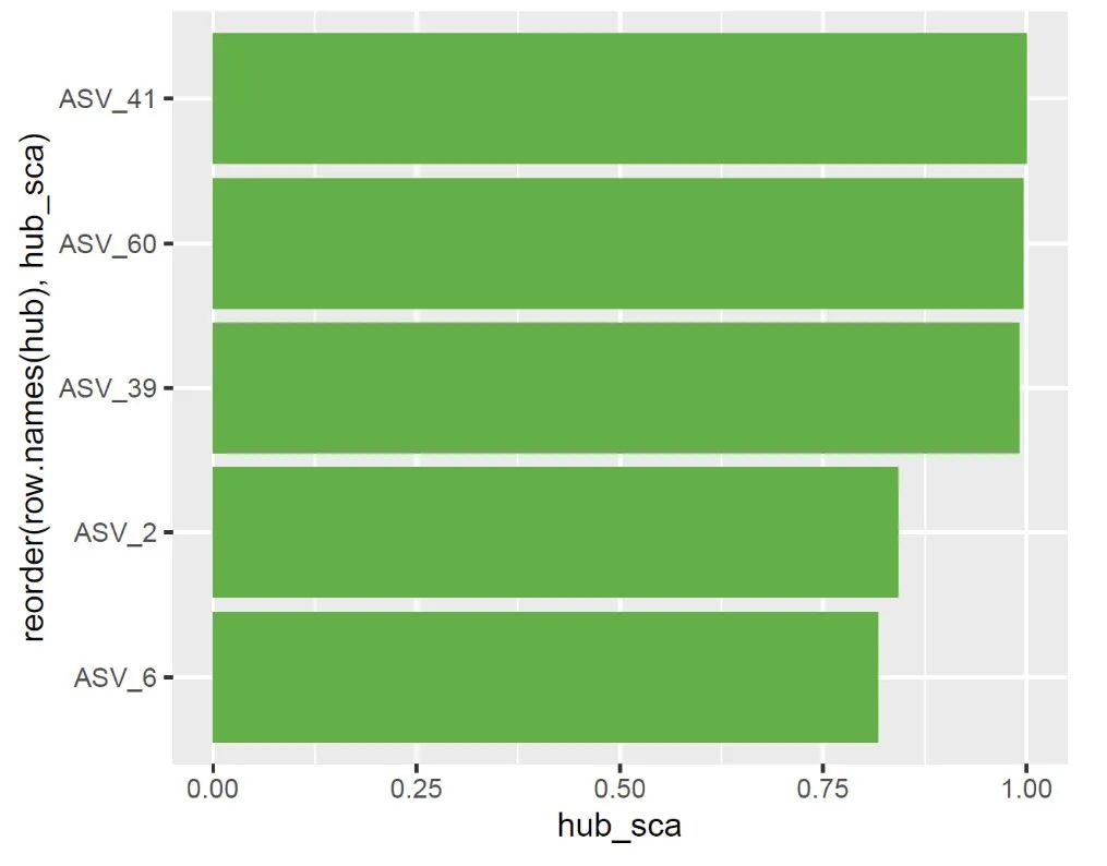
节点性质计算
nodepro = node_properties(igraph)
head(nodepro)
value
num.edges(L) 1.736000e+03
num.pos.edges 1.247000e+03
num.neg.edges 4.890000e+02
num.vertices(n) 6.010000e+02
Connectance(edge_density) 9.628397e-03
average.degree(Average K) 5.777038e+00
average.path.length 4.750325e+00
diameter 1.263110e+01
edge.connectivity 0.000000e+00
mean.clustering.coefficient(Average.CC) 2.909496e-01
no.clusters 5.100000e+01
centralization.degree 7.203827e-02
centralization.betweenness 8.584971e-02
centralization.closeness 2.737148e-03
RM(relative.modularity) -6.258599e-01
the.number.of.keystone.nodes 1.100000e+02扩展-关键OTU挑选
Hub节点是在网络中与其他节点连接较多的节点,Hub微生物就是与其他微生物联系较为紧密的微生物,可以称之为关键微生物(keystone)
hub = hub_score(igraph)$vector %>%
  sort(decreasing = TRUE) %>%
  head(5) %>%
  as.data.frame()

colnames(hub) = "hub_sca"

ggplot(hub) +
  geom_bar(aes(x = hub_sca,y = reorder(row.names(hub),hub_sca)),stat = "identity",fill = "#4DAF4A")
对应随机网络构建和网络参数比对
result = random_Net_compate(igraph = igraph, type = "gnm", step = 100, netName = layout)
p1 = result[[1]]
sum_net = result[[4]]
p1
head(sum_net)
微生物组网络pipeline分析
使用network函数运行微生物网络全套分析:
使用OTU数量建议少于250个,如果OTU数量为250个,同时计算zipi,整个运算过程为3-5min。
data("ps16s")
path = "./result_micro_200/"
dir.create(path)

result = network(ps = ps16s,
                 N = 200,
                layout_net = "model_Gephi.2",
                 r.threshold=0.6,
                 p.threshold=0.05,
                 label = FALSE,
                 path = path,
                 zipi = TRUE)

# 多组网络绘制到一个面板
p = result[[1]]
p
# 全部样本网络参数比对
data = result[[2]]

plotname1 = paste(path,"/network_all.jpg",sep = "")
ggsave(plotname1, p,width = 48,height = 16,dpi = 72)

plotname1 = paste(path,"/network_all.pdf",sep = "")
ggsave(plotname1, p,width = 48,height = 16)

tablename <- paste(path,"/co-occurrence_Grobel_net",".csv",sep = "")
write.csv(data,tablename)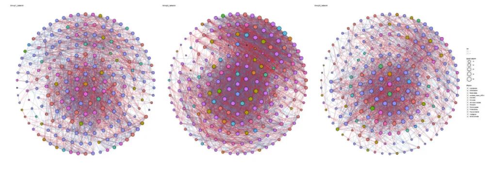
微生物网络-大网络
使用model_maptree2布局计算微生物大网络。
大网络运算时间会比较长,这里我没有计算zipi,用时5min完成全部运行。
N=0,代表用全部的OTU进行计算。
3000个OTU不计算zipi全套需要18min。
path = "./result_big_1000/"
dir.create(path)

result = network.2(ps = ps16s,
                 N = 1000,
                 big = TRUE,
                 maxnode = 5,
                 select_layout = TRUE,
                  layout_net = "model_maptree2",
                 r.threshold=0.4,
                 p.threshold=0.01,
                 label = FALSE,
                 path = path,
                 zipi = FALSE)

# 多组网络绘制到一个面板
p = result[[1]]
# 全部样本网络参数比对
data = result[[2]]
num= 3
# plotname1 = paste(path,"/network_all.jpg",sep = "")
# ggsave(plotname1, p,width = 16*num,height = 16,dpi = 72)

plotname1 = paste(path,"/network_all.pdf",sep = "")
ggsave(plotname1, p,width = 10*num,height = 10,limitsize = FALSE)

tablename <- paste(path,"/co-occurrence_Grobel_net",".csv",sep = "")
write.csv(data,tablename)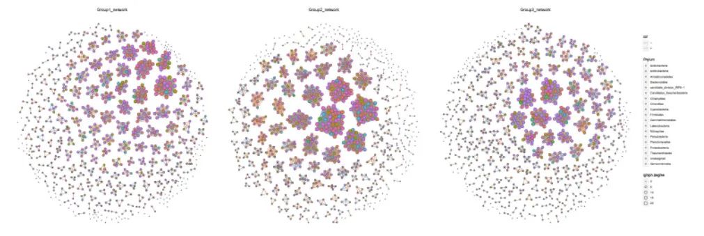
使用model_igraph布局绘制微生物大网络
path = "./result_1000_igraph/"
dir.create(path)
map = sample_data(ps16s)
map$Group = "one"
sample_data(ps16s) = map
result = network.2(ps = ps16s,
                 N = 1000,
                 big = TRUE,
                 maxnode = 5,
                 select_layout = TRUE,
                  layout_net = "model_igraph",
                 r.threshold=0.4,
                 p.threshold=0.01,
                 label = FALSE,
                 path = path,
                 zipi = FALSE)

# 多组网络绘制到一个面板
p = result[[1]]
# 全部样本网络参数比对
data = result[[2]]
num= 3
# plotname1 = paste(path,"/network_all.jpg",sep = "")
# ggsave(plotname1, p,width = 16*num,height = 16,dpi = 72)

plotname1 = paste(path,"/network_all.pdf",sep = "")
ggsave(plotname1, p,width = 16*num,height = 16,limitsize = FALSE)

tablename <- paste(path,"/co-occurrence_Grobel_net",".csv",sep = "")
write.csv(data,tablename)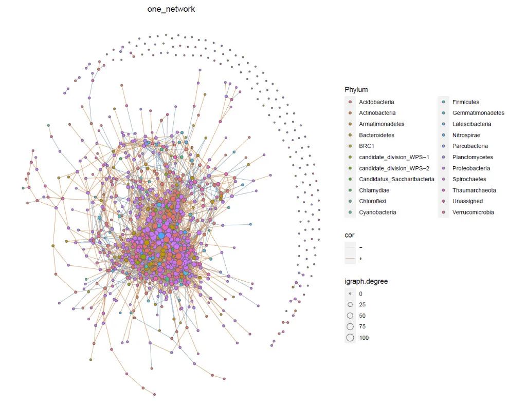
跨域网络pipeline分析
细菌,真菌,环境因子三者跨域网络
#--细菌和环境因子的网络#--------
Envnetplot<- paste("./16s_ITS_Env_network",sep = "")
dir.create(Envnetplot)

ps16s =ps16s%>% ggClusterNet::scale_micro()
psITS = psITS%>% ggClusterNet::scale_micro()

library(phyloseq)
#--细菌和真菌ps对象中的map文件要一样
ps.merge <- ggClusterNet::merge16S_ITS(ps16s = ps16s,
                                       psITS= psITS,
                         NITS = 200,
                         N16s = 200)

map =  phyloseq::sample_data(ps.merge)
head(map)
map$Group = "one"
phyloseq::sample_data(ps.merge) <- map

#--环境因子导入
data1 = env
envRDA  = data.frame(row.names = env$ID,env[,-1])

envRDA.s = vegan::decostand(envRDA,"hellinger")
data1[,-1] = envRDA.s

Gru = data.frame(ID = colnames(env)[-1],group = "env" )
head(Gru)

library(sna)
library(ggClusterNet)
library(igraph)

result <- ggClusterNet::corBionetwork(ps = ps.merge,
                        N = 0,
                        r.threshold = 0.4, # 相关阈值
                        p.threshold = 0.05,
                        big = T,
                        group = "Group",
                        env = data1, # 环境指标表格
                        envGroup = Gru,# 环境因子分组文件表格
                        # layout = "fruchtermanreingold",
                        path = Envnetplot,# 结果文件存储路径
                        fill = "Phylum", # 出图点填充颜色用什么值
                        size = "igraph.degree", # 出图点大小用什么数据
                        scale = TRUE, # 是否要进行相对丰度标准化
                        bio = TRUE, # 是否做二分网络
                        zipi = F, # 是否计算ZIPI
                        step = 100, # 随机网络抽样的次数
                        width = 18,
                        label = TRUE,
                        height = 10
)

p = result[[1]]
p
# 全部样本网络参数比对
data = result[[2]]
plotname1 = paste(Envnetplot,"/network_all.jpg",sep = "")
ggsave(plotname1, p,width = 15,height = 12,dpi = 72)
# plotname1 = paste(Envnetplot,"/network_all.png",sep = "")
# ggsave(plotname1, p,width = 10,height = 8,dpi = 72)
plotname1 = paste(Envnetplot,"/network_all.pdf",sep = "")
ggsave(plotname1, p,width = 15,height = 12)
tablename <- paste(Envnetplot,"/co-occurrence_Grobel_net",".csv",sep = "")
write.csv(data,tablename)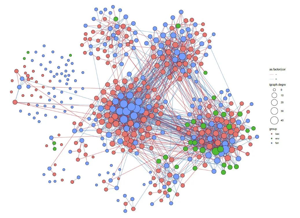
细菌环境因子跨域网络
#--细菌-环境因子网络#-----
Envnetplot<- paste("./16s_Env_network",sep = "")
dir.create(Envnetplot)
# ps16s = ps0 %>% ggClusterNet::scale_micro()
psITS = NULL
library(phyloseq)
#--细菌和真菌ps对象中的map文件要一样
ps.merge <- ggClusterNet::merge16S_ITS(ps16s = ps16s,
                                       psITS = NULL,
                                       N16s = 500)
ps.merge
map =  phyloseq::sample_data(ps.merge)
head(map)
map$Group = "one"
phyloseq::sample_data(ps.merge) <- map

data1 = env
envRDA.s = vegan::decostand(envRDA,"hellinger")
data1[,-1] = envRDA.s

Gru = data.frame(ID = colnames(env)[-1],group = "env" )
head(Gru)

# library(sna)
# library(ggClusterNet)
# library(igraph)

result <- ggClusterNet::corBionetwork(ps = ps.merge,
                                      N = 0,
                                      r.threshold = 0.4, # 相关阈值
                                      p.threshold = 0.05,
                                      big = T,
                                      group = "Group",
                                      env = data1, # 环境指标表格
                                      envGroup = Gru,# 环境因子分组文件表格
                                      # layout = "fruchtermanreingold",
                                      path = Envnetplot,# 结果文件存储路径
                                      fill = "Phylum", # 出图点填充颜色用什么值
                                      size = "igraph.degree", # 出图点大小用什么数据
                                      scale = TRUE, # 是否要进行相对丰度标准化
                                      bio = TRUE, # 是否做二分网络
                                      zipi = F, # 是否计算ZIPI
                                      step = 100, # 随机网络抽样的次数
                                      width = 18,
                                      label = TRUE,
                                      height = 10
)

p = result[[1]]
p
# 全部样本网络参数比对
data = result[[2]]
plotname1 = paste(Envnetplot,"/network_all.jpg",sep = "")
ggsave(plotname1, p,width = 13,height = 12,dpi = 72)

plotname1 = paste(Envnetplot,"/network_all.pdf",sep = "")
ggsave(plotname1, p,width = 13,height = 12)
tablename <- paste(Envnetplot,"/co-occurrence_Grobel_net",".csv",sep = "")
write.csv(data,tablename)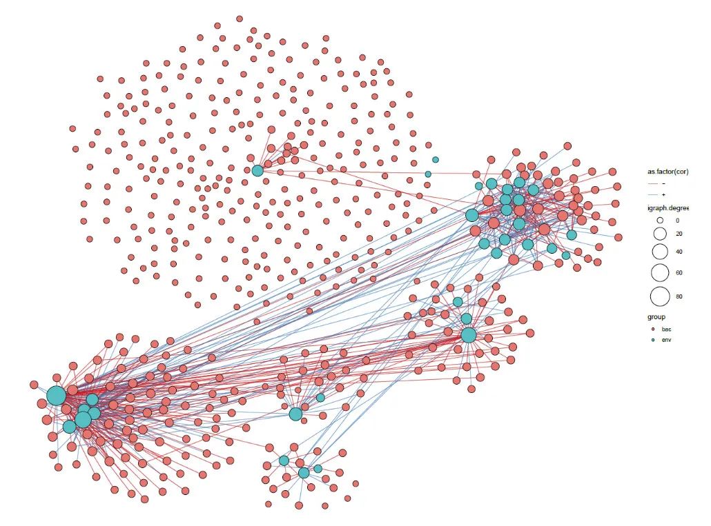
细菌真菌跨越网络
#---细菌和真菌OTU网络-域网络-二分网络#-------
# 仅仅关注细菌和真菌之间的相关,不关注细菌内部和真菌内部相关

Envnetplot<- paste("./16S_ITS_network",sep = "")
dir.create(Envnetplot)

data(psITS)
#--细菌和真菌ps对象中的map文件要一样
ps.merge <- ggClusterNet::merge16S_ITS(ps16s = ps16s,
                                       psITS = psITS,
                                       N16s = 500,
                                       NITS = 500
)

ps.merge

map =  phyloseq::sample_data(ps.merge)

head(map)
map$Group = "one"
phyloseq::sample_data(ps.merge) <- map

data =  data.frame(ID = c("fun_ASV_205","fun_ASV_316","fun_ASV_118"),
                   c("Coremode","Coremode","Coremode"))

# source("F:/Shared_Folder/Function_local/R_function/my_R_packages/ggClusterNet/R/corBionetwork2.R")

result <- corBionetwork(ps = ps.merge,
                        N = 0,
                        lab = data,
                        r.threshold = 0.8, # 相关阈值
                        p.threshold = 0.05,
                        group = "Group",
                        # env = data1, # 环境指标表格
                        # envGroup = Gru,# 环境因子分组文件表格
                        # layout = "fruchtermanreingold",
                        path = Envnetplot,# 结果文件存储路径
                        fill = "Phylum", # 出图点填充颜色用什么值
                        size = "igraph.degree", # 出图点大小用什么数据
                        scale = TRUE, # 是否要进行相对丰度标准化
                        bio = TRUE, # 是否做二分网络
                        zipi = F, # 是否计算ZIPI
                        step = 100, # 随机网络抽样的次数
                        width = 12,
                        label = TRUE,
                        height = 10,
                        big = TRUE,
                        select_layout = TRUE,
                        layout_net = "model_maptree2",
                        clu_method = "cluster_fast_greedy"


)

tem <- model_maptree(cor =result[[5]],
                     method = "cluster_fast_greedy",
                     seed = 12
)
node_model = tem[[2]]
head(node_model)

p = result[[1]]
p
# 全部样本网络参数比对
data = result[[2]]

plotname1 = paste(Envnetplot,"/network_all.pdf",sep = "")
ggsave(plotname1, p,width = 20,height = 19)
tablename <- paste(Envnetplot,"/co-occurrence_Grobel_net",".csv",sep = "")
write.csv(data,tablename)
tablename <- paste(Envnetplot,"/node_model_imformation",".csv",sep = "")
write.csv(node_model,tablename)

tablename <- paste(Envnetplot,"/nodeG_plot",".csv",sep = "")
write.csv(result[[4]],tablename)
tablename <- paste(Envnetplot,"/edge_plot",".csv",sep = "")
write.csv(result[[3]],tablename)
tablename <- paste(Envnetplot,"/cor_matrix",".csv",sep = "")
write.csv(result[[5]],tablename)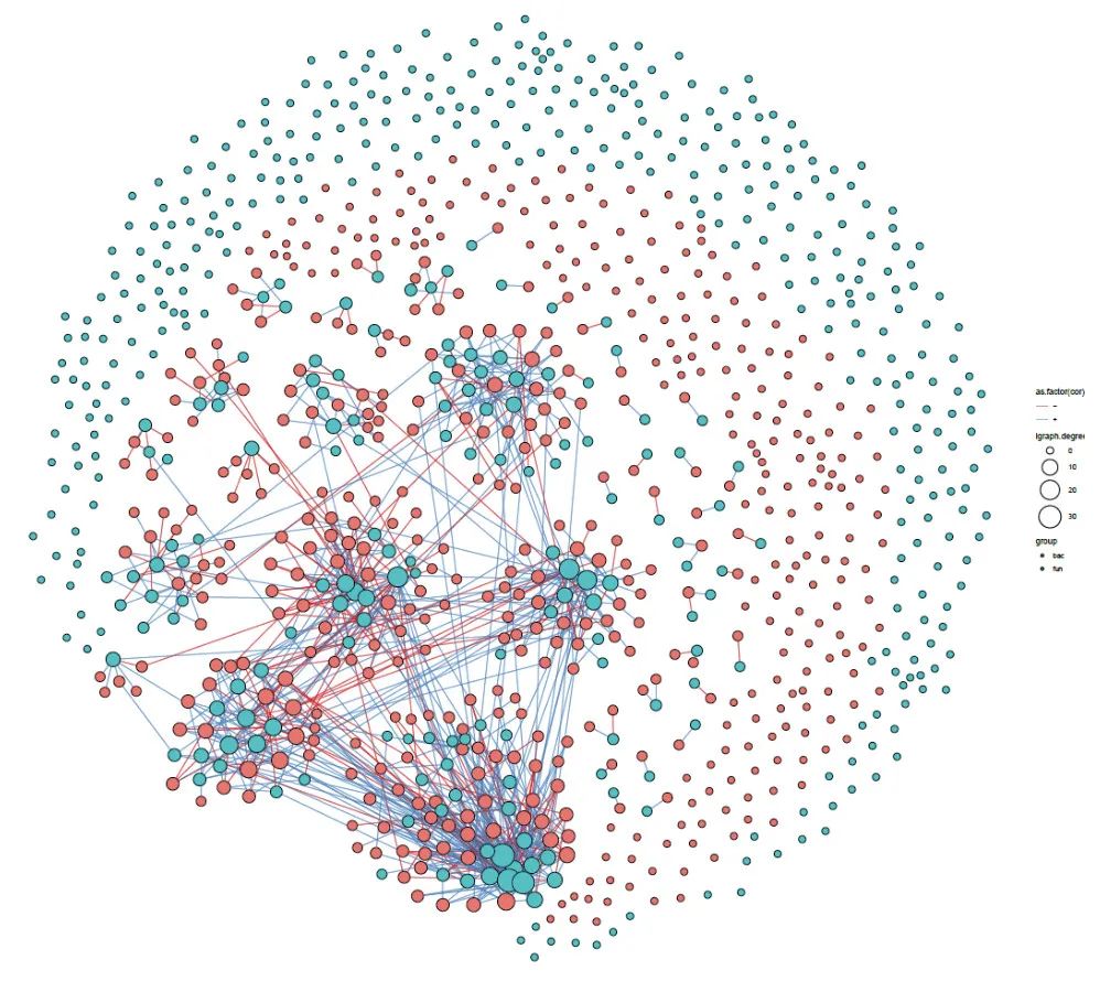
基于属水平绘制跨域网络-网络模块与环境因子相关等
#--细菌真菌任意分类水平跨域网络#----------
library(tidyverse)
# res1path = "result_and_plot/Micro_and_other_index_16s/"
Envnetplot<- paste("./16S_ITS_network_Genus",sep = "")
dir.create(Envnetplot)
#--细菌和真菌ps对象中的map文件要一样
ps.merge <- merge16S_ITS(ps16s = ps16s,
                         psITS = psITS,
                         N16s = 500,
                         NITS = 500
)
ps.merge
map =  phyloseq::sample_data(ps.merge)
head(map)
map$Group = "one"
phyloseq::sample_data(ps.merge) <- map
tem.0 = ps.merge %>% tax_glom_wt(ranks = "Genus")
tax = tem.0 %>% vegan_tax() %>%
  as.data.frame()
head(tax)

data =  data.frame(ID = c("Acaulium","Acidocella","Acrobeloides"),
                   c("Acaulium","Acidocella","Acrobeloides"))

result <- corBionetwork(ps = tem.0,
                        N = 0,
                        lab = data,
                        r.threshold = 0.6, # 相关阈值
                        p.threshold = 0.05,
                        group = "Group",
                        # env = data1, # 环境指标表格
                        # envGroup = Gru,# 环境因子分组文件表格
                        # layout = "fruchtermanreingold",
                        path = Envnetplot,# 结果文件存储路径
                        fill = "Phylum", # 出图点填充颜色用什么值
                        size = "igraph.degree", # 出图点大小用什么数据
                        scale = TRUE, # 是否要进行相对丰度标准化
                        bio = TRUE, # 是否做二分网络
                        zipi = F, # 是否计算ZIPI
                        step = 100, # 随机网络抽样的次数
                        width = 12,
                        label = TRUE,
                        height = 10,
                        big = TRUE,
                        select_layout = TRUE,
                        layout_net = "model_maptree2",
                        clu_method = "cluster_fast_greedy"


)

tem <- model_maptree(cor =result[[5]],
                     method = "cluster_fast_greedy",
                     seed = 12
)
node_model = tem[[2]]
head(node_model)

library(WGCNA)
otu = tem.0 %>% vegan_otu() %>%
  as.data.frame()
node_model = node_model[match(colnames(otu),node_model$ID),]

MEList = moduleEigengenes(otu, colors = node_model$group)
MEs = MEList$eigengenes

nGenes = ncol(otu)
nSamples = nrow(otu)
moduleTraitCor = cor(MEs, envRDA, use = "p")
moduleTraitPvalue = corPvalueStudent(moduleTraitCor, nSamples)

#sizeGrWindow(10,6)
pdf(file=paste(Envnetplot,"/","Module-env_relationships.pdf",sep = ""),width=10,height=6)
# Will display correlations and their p-values
textMatrix = paste(signif(moduleTraitCor, 2), "\n(",
                   signif(moduleTraitPvalue, 1), ")", sep = "")

dim(textMatrix) = dim(moduleTraitCor)
par(mar = c(6, 8.5, 3, 3))
# Display the correlation values within a heatmap plot
labeledHeatmap(Matrix = moduleTraitCor,
               xLabels = names(envRDA),
               yLabels = names(MEs),
               ySymbols = names(MEs),
               colorLabels = FALSE,
               colors = greenWhiteRed(50),
               textMatrix = textMatrix,
               setStdMargins = FALSE,
               cex.text = 0.5,
               zlim = c(-1,1),
               main = paste("Module-trait relationships"))
dev.off()

p = result[[1]]
p
# 全部样本网络参数比对
data = result[[2]]

plotname1 = paste(Envnetplot,"/network_all.pdf",sep = "")
ggsave(plotname1, p,width = 10,height = 10)
tablename <- paste(Envnetplot,"/co-occurrence_Grobel_net",".csv",sep = "")
write.csv(data,tablename)

tablename <- paste(Envnetplot,"/nodeG_plot",".csv",sep = "")
write.csv(result[[4]],tablename)
tablename <- paste(Envnetplot,"/edge_plot",".csv",sep = "")
write.csv(result[[3]],tablename)
tablename <- paste(Envnetplot,"/cor_matrix",".csv",sep = "")
write.csv(result[[5]],tablename)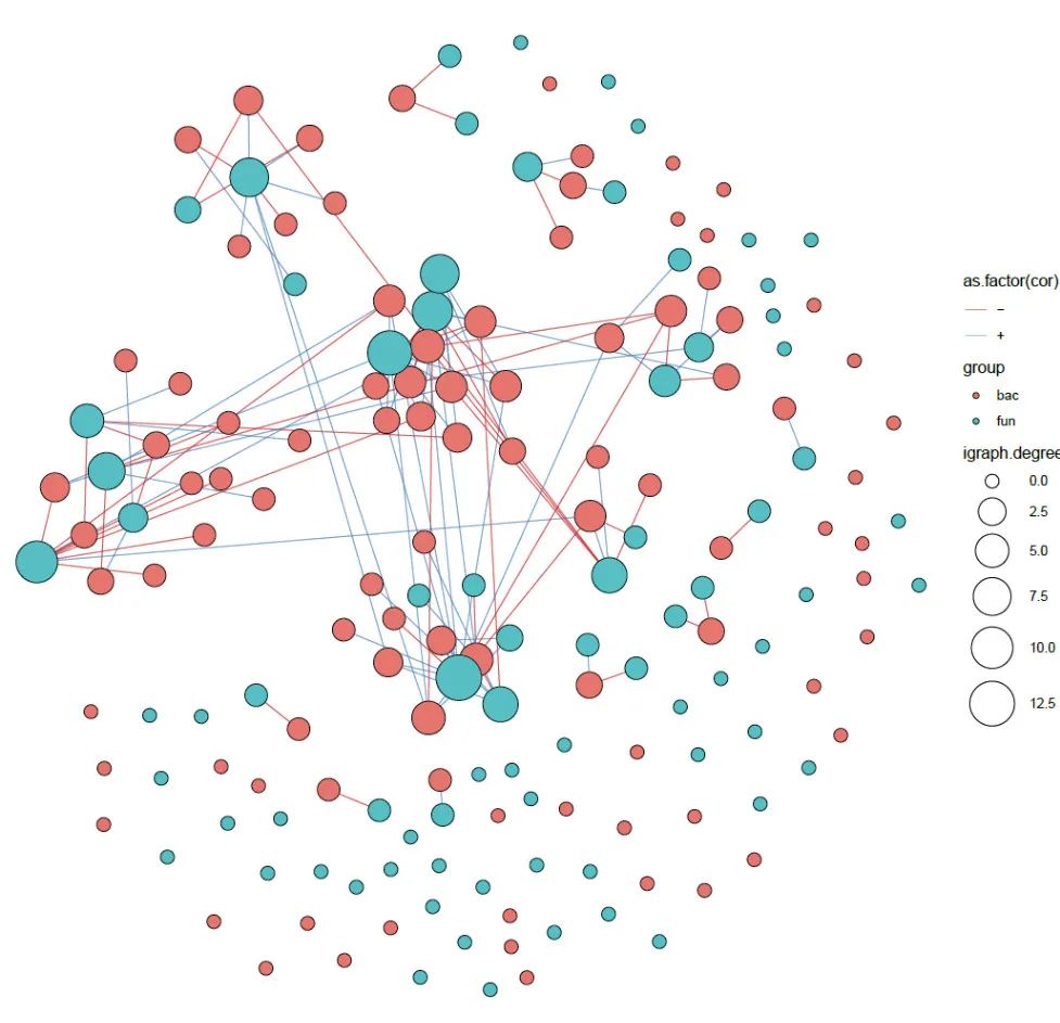
引文:Tao Wen, Penghao Xie, Shengdie Yang, Guoqing Niu, Xiaoyu Liu, Zhexu Ding, Chao Xue, Yong-Xin Liu, Qirong Shen, Jun Yuan. 2022. ggClusterNet: An R package for microbiome network analysis and modularity-based multiple network layouts. iMeta 1: e32. https://doi.org/10.1002/imt2.32

“iMeta” 是由威立、肠菌分会和本领域数百位华人科学家合作出版的开放获取期刊,主编由中科院微生物所刘双江研究员和荷兰格罗宁根大学傅静远教授担任。目的是发表原创研究、方法和综述以促进宏基因组学、微生物组和生物信息学发展。目标是发表前10%(IF > 15)的高影响力论文。期刊特色包括视频投稿、可重复分析、图片打磨、青年编委、前3年免出版费、50万用户的社交媒体宣传等。2022年2月正式创刊发行!
联系我们
iMeta主页:http://www.imeta.science
出版社:https://onlinelibrary.wiley.com/journal/2770596x
投稿:https://mc.manuscriptcentral.com/imeta
邮箱:office@imeta.science
微信公众号
iMeta
往期精品(点击图片直达文字对应教程)
|
|
|
|
|
|
|
|
|
|
|
|
|
|
|
|
|
|
|
|
|
|
|
|
|
|
|
|


后台回复“生信宝典福利第一波”或点击阅读原文获取教程合集