【Python】多图形混合排版，如何在Matplotlib/Seaborn中实现？

• 通过|、/轻松实现图形排列；
• 比matplotlib、seaborn等自带子图功能更加灵活;
• 灵感源于R中的_patchwork。

更多关于图形拼接文章：
ProPlot弥补Matplotlib这9大缺陷
Matplotlib-多子图绘制

在Matplotlib中使用patchworklib拼图

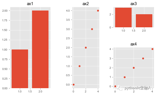
主要使用pw.Brick方法和savefig方法。

import patchworklib as pw
import matplotlib.pyplot as plt
plt.style.use('ggplot')

#绘制子图1
ax1 = pw.Brick(figsize=(1, 2))  #每个子图调用pw.Brick方法
ax1.bar([1, 2], [1, 2])
ax1.set_title("ax1")

#绘制子图2
ax2 = pw.Brick(figsize=(1, 3))
ax2.scatter(range(5), range(5))
ax2.set_title("ax2")

#绘制子图3
ax3 = pw.Brick(figsize=(2, 1))
ax3.bar([2, 1], [2, 3])
ax3.set_title("ax3")

#绘制子图4
ax4 = pw.Brick(figsize=(2, 2))
ax4.scatter(range(5), range(5))
ax4.set_title("ax4")

#拼图
ax1234 = (ax1 | ax2) | (ax3 / ax4)
ax1234.savefig()  #类似plt.show()

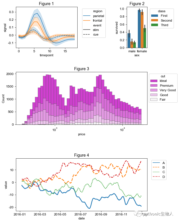
在Seaborn中使用patchworklib拼图 (Axes水平)

和前面Matplotlib中一样，主要使用pw.Brick方法和savefig方法。

关于Axes水平和Figure水平差异，请参考👉Matplotlib太臃肿，试试Seaborn

import pandas as pd
import seaborn as sns
import patchworklib as pw

#ax1
ax1 = pw.Brick(figsize=(3,2)) #每个子图调用pw.Brick方法
fmri = sns.load_dataset("fmri")
sns.lineplot(x="timepoint", y="signal", hue="region", style="event", data=fmri, ax=ax1)
ax1.move_legend(new_loc='upper left', bbox_to_anchor=(1.05, 1.0))
ax1.set_title("ax1")

#ax2
ax2 = pw.Brick(figsize=(1,2))
titanic = sns.load_dataset("titanic")
sns.barplot(x="sex", y="survived", hue="class", data=titanic, ax=ax2)
ax2.move_legend(new_loc='upper left', bbox_to_anchor=(1.05, 1.0))
ax2.set_title("ax2")

#ax3
ax3 = pw.Brick(figsize=(5,2))
diamonds = sns.load_dataset("diamonds")
sns.histplot(diamonds, x="price", hue="cut", multiple="stack", palette="light:m_r", edgecolor=".3", linewidth=.5, log_scale=True, ax = ax3)
ax3.move_legend(new_loc='upper left', bbox_to_anchor=(1.0, 1.0))
ax3.set_title("ax3")

#ax4
ax4 = pw.Brick(figsize=(6,2))
tips = sns.load_dataset("tips")
sns.violinplot(data=tips, x="day", y="total_bill", hue="smoker",split=True, inner="quart", linewidth=1, palette={"Yes": "b", "No": ".85"}, ax=ax4)
ax4.move_legend("upper left", bbox_to_anchor=(1.02, 1.0))
ax4.set_title("ax4")

#ax5
ax5    = pw.Brick(figsize=(5,2))
rs     = np.random.RandomState(365)
values = rs.randn(365, 4).cumsum(axis=0)
dates  = pd.date_range("1 1 2016", periods=365, freq="D")
data   = pd.DataFrame(values, dates, columns=["A", "B", "C", "D"])
data = data.rolling(7).mean()
sns.lineplot(data=data, palette="tab10", linewidth=2.5, ax=ax5)
ax5.set_xlabel("date")
ax5.set_ylabel("value")
ax5.move_legend("upper left", bbox_to_anchor=(1.02, 1.0))
ax5.set_title("ax5")

#拼图
ax12345 = (ax1|ax2)/(ax3/ax4)/(ax5)
ax12345.savefig()

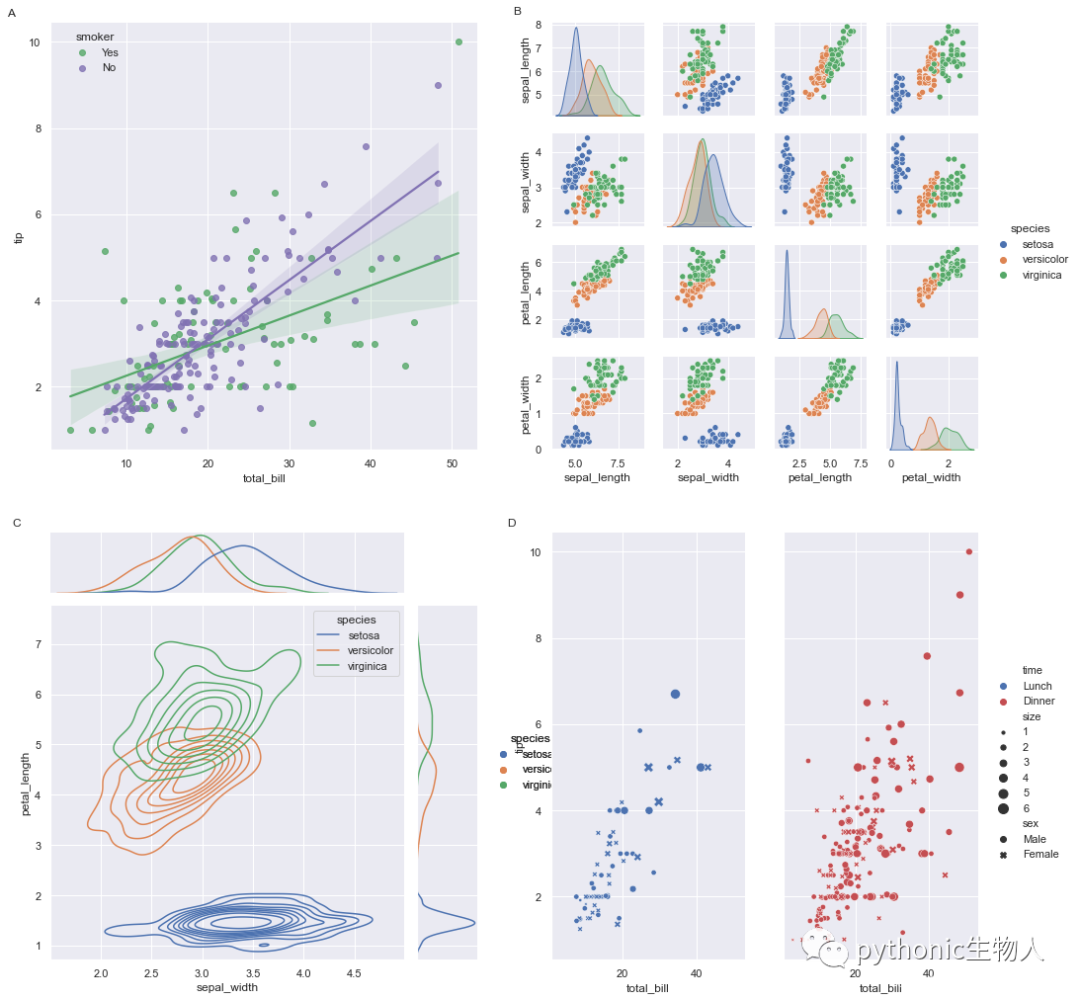
在Seaborn中使用patchworklib拼图 (Figure水平)

此处主要使用load_seabrongrid方法和pw.overwrite_axisgrid()方法。

import matplotlib
import seaborn as sns
import patchworklib as pw 

pw.overwrite_axisgrid() # 使用pw.load_seagorngrid，必须先开启pw.overwrite_axisgrid方法 

iris = sns.load_dataset("iris")
tips = sns.load_dataset("tips")

# An lmplot
g0 = sns.lmplot(x="total_bill", y="tip", hue="smoker", data=tips, 
                palette=dict(Yes="g", No="m"))
g0 = pw.load_seaborngrid(g0, label="g0") #每个子图使用使用pw.load_seagorngrid方法

# A Pairplot
g1 = sns.pairplot(iris, hue="species")
g1 = pw.load_seaborngrid(g1, label="g1", figsize=(6,6))

# A relplot
g2 = sns.relplot(data=tips, x="total_bill", y="tip", col="time", hue="time", 
                 size="size", style="sex", palette=["b", "r"], sizes=(10, 100))
g2.set_titles("")
g2 = pw.load_seaborngrid(g2, label="g2")

# A JointGrid
g3 = sns.jointplot(x="sepal_width", y="petal_length", data=iris,hue="species",
                   kind="kde", space=0, color="g")

g3 = pw.load_seaborngrid(g3, label="g3", labels=["joint","marg_x","marg_y"])

#个性化设置
g0.case.set_title('A', x=0, y=1.0, loc="right")
g0.move_legend("upper left", bbox_to_anchor=(0.1,1.0))
g1.case.set_title('B', x=0, y=1.0, loc="right")
g3.case.set_title('C', x=0, y=1.0, loc="right")
g2.case.set_title('D', x=0, y=1.0, loc="right")

#拼图
(((g0/g3)["g0"]|g1)["g1"]/g2).savefig()

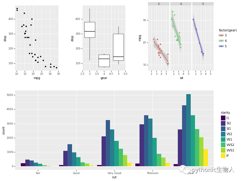
在plotnine中使用patchworklib拼图

此处主要使用pw.load_ggplot方法。关于plotnine👉plotnine!!!终于可以在Python中使用ggplot2

import patchworklib as pw 
from plotnine import * 
from plotnine.data import *  

g1 = (ggplot(mtcars) + geom_point(aes("mpg", "disp"))) 
g1 = pw.load_ggplot(g1, figsize=(2,3)) #每个子图重复使用pw.load_ggplot方法

g2 = (ggplot(mtcars) + geom_boxplot(aes("gear", "disp", group="gear"))) 
g2 = pw.load_ggplot(g2, figsize=(2,3))

g3 = (ggplot(mtcars, aes('wt', 'mpg', color='factor(gear)')) + geom_point() + stat_smooth(method='lm') + facet_wrap('~gear')) 
g3 = pw.load_ggplot(g3, figsize=(3,3))

g4 = (ggplot(data=diamonds) + geom_bar(mapping=aes(x="cut", fill="clarity"), position="dodge"))  
g4 = pw.load_ggplot(g4, figsize=(5,2))

#拼图
g1234 = (g1|g2|g3)/g4 
g1234.savefig()

ref: https://github.com/ponnhide/patchworklib