
贝叶斯推理三种方法:MCMC 、HMC和SBI
共 8222字,需浏览 17分钟
· 2022-11-18

来源:Deephub Imba 本文约3200字,建议阅读10分钟 本文整理的是作者最近在普林斯顿的一个研讨会上做的演讲幻灯片,这样可以阐明为什么贝叶斯方法不仅在逻辑上是合理的,而且使用起来也很简单。
对许多人来说,贝叶斯统计仍然有些陌生。因为贝叶斯统计中会有一些主观的先验,在没有测试数据的支持下了解他的理论还是有一些困难的。本文整理的是作者最近在普林斯顿的一个研讨会上做的演讲幻灯片,这样可以阐明为什么贝叶斯方法不仅在逻辑上是合理的,而且使用起来也很简单。这里将以三种不同的方式实现相同的推理问题。
数据
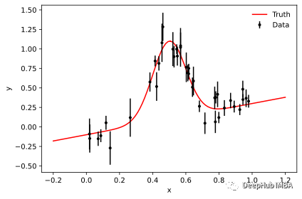
我们的例子是在具有倾斜背景的噪声数据中找到峰值的问题,这可能出现在粒子物理学和其他多分量事件过程中。
首先生成数据:
%matplotlib inline%config InlineBackend.figure_format = 'svg'import matplotlib.pyplot as pltimport numpy as npdef signal(theta, x):l, m, s, a, b = thetapeak = l * np.exp(-(m-x)**2 / (2*s**2))background = a + b*xreturn peak + backgrounddef plot_results(x, y, y_err, samples=None, predictions=None):fig = plt.figure()ax = fig.gca()ax.errorbar(x, y, yerr=y_err, fmt=".k", capsize=0, label="Data")x0 = np.linspace(-0.2, 1.2, 100)ax.plot(x0, signal(theta, x0), "r", label="Truth", zorder=0)if samples is not None:inds = np.random.randint(len(samples), size=50)for i,ind in enumerate(inds):theta_ = samples[ind]if i==0:label='Posterior'else:label=Noneax.plot(x0, signal(theta_, x0), "C0", alpha=0.1, zorder=-1, label=label)elif predictions is not None:for i, pred in enumerate(predictions):if i==0:label='Posterior'else:label=Noneax.plot(x0, pred, "C0", alpha=0.1, zorder=-1, label=label)ax.legend(frameon=False)ax.set_xlabel("x")ax.set_ylabel("y")fig.tight_layout()plt.close();return fig# random x locationsN = 40np.random.seed(0)x = np.random.rand(N)# evaluate the true model at the given x valuestheta = [1, 0.5, 0.1, -0.1, 0.4]y = signal(theta, x)# add heteroscedastic Gaussian uncertainties only in y directiony_err = np.random.uniform(0.05, 0.25, size=N)y = y + np.random.normal(0, y_err)# plotplot_results(x, y, y_err)
有了数据我们可以介绍三种方法了。
马尔可夫链蒙特卡罗 Markov Chain Monte Carlo
emcee是用纯python实现的,它只需要评估后验的对数作为参数θ的函数。这里使用对数很有用,因为它使指数分布族的分析评估更容易,并且因为它更好地处理通常出现的非常小的数字。
import emceedef log_likelihood(theta, x, y, yerr):y_model = signal(theta, x)chi2 = (y - y_model)**2 / (yerr**2)return np.sum(-chi2 / 2)def log_prior(theta):if all(theta > -2) and (theta[2] > 0) and all(theta < 2):return 0return -np.infdef log_posterior(theta, x, y, yerr):lp = log_prior(theta)if np.isfinite(lp):lp += log_likelihood(theta, x, y, yerr)return lp# create a small ball around the MLE the initialize each walkernwalkers, ndim = 30, 5theta_guess = [0.5, 0.6, 0.2, -0.2, 0.1]pos = theta_guess + 1e-4 * np.random.randn(nwalkers, ndim)# run emceesampler = emcee.EnsembleSampler(nwalkers, ndim, log_posterior, args=(x, y, y_err))sampler.run_mcmc(pos, 10000, progress=True);
结果如下:
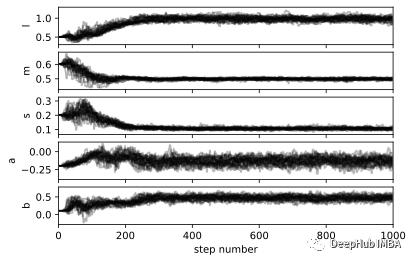
100%|██████████| 10000/10000我们应该始终检查生成的链,确定burn-in period,并且需要人肉观察平稳性:
fig, axes = plt.subplots(ndim, sharex=True)mcmc_samples = sampler.get_chain()labels = ["l", "m", "s", "a", "b"]for i in range(ndim):ax = axes[i]ax.plot(mcmc_samples[:, :, i], "k", alpha=0.3, rasterized=True)ax.set_xlim(0, 1000)ax.set_ylabel(labels[i])axes[-1].set_xlabel("step number");
现在我们需要细化链因为我们的样本是相关的。这里有一个方法来计算每个参数的自相关,我们可以将所有的样本结合起来:
tau = sampler.get_autocorr_time()print("Autocorrelation time:", tau)mcmc_samples = sampler.get_chain(discard=300, thin=np.int32(np.max(tau)/2), flat=True)print("Remaining samples:", mcmc_samples.shape)
#结果Autocorrelation time: [122.51626866 75.87228105 137.195509 54.63572513 79.0331587 ]Remaining samples: (4260, 5)
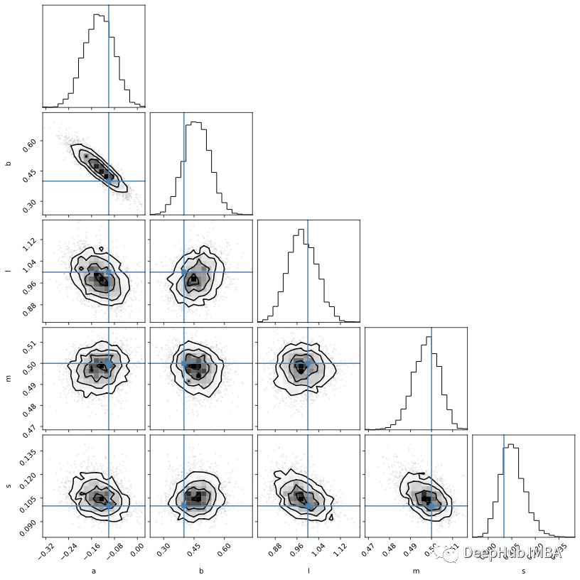
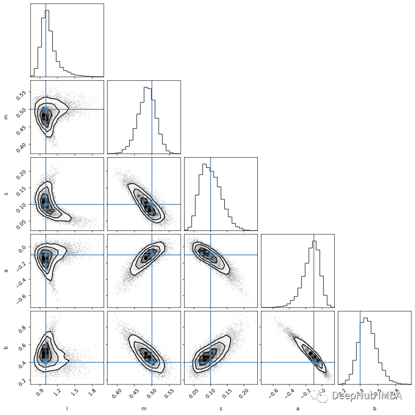
emcee 的创建者 Dan Foreman-Mackey 还提供了这一有用的包corner来可视化样本:
import cornercorner.corner(mcmc_samples, labels=labels, truths=theta);
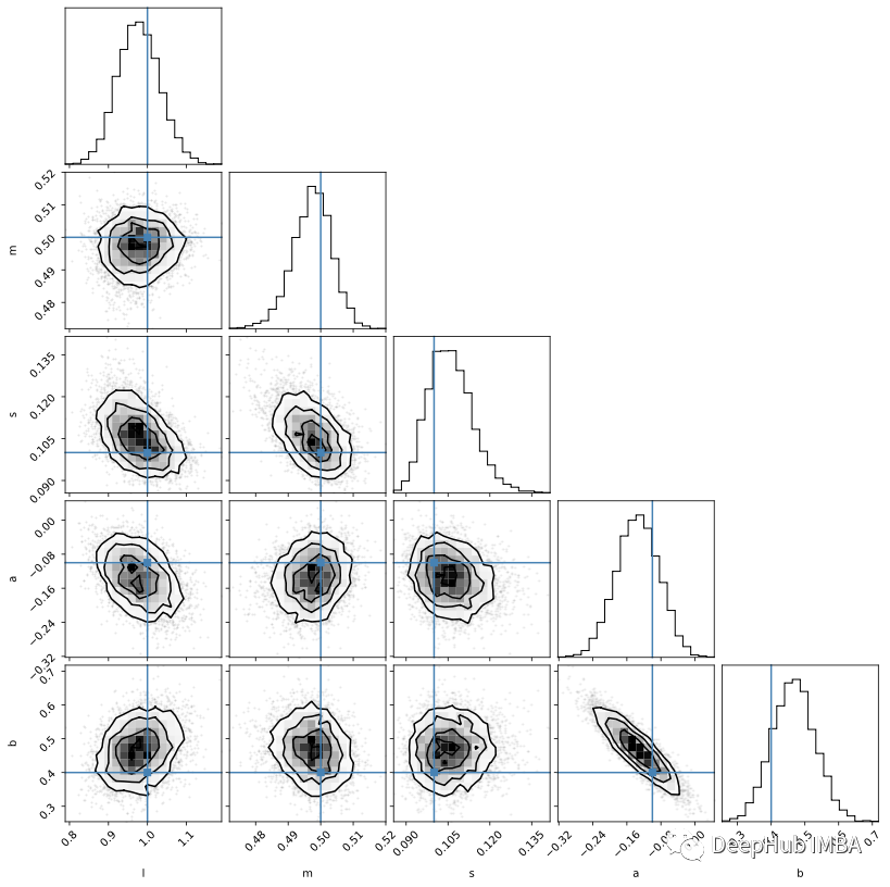
虽然后验样本是推理的主要依据,但参数轮廓本身却很难解释。但是使用样本来生成新数据则要简单得多,因为这个可视化我们对数据空间有更多的理解。以下是来自50个随机样本的模型评估:
plot_results(x, y, y_err, samples=mcmc_samples)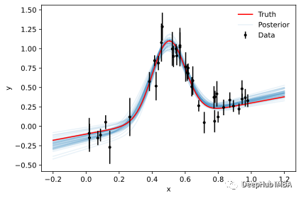
哈密尔顿蒙特卡洛 Hamiltonian Monte Carlo
梯度在高维设置中提供了更多指导。为了实现一般推理,我们需要一个框架来计算任意概率模型的梯度。这里关键的本部分是自动微分,我们需要的是可以跟踪参数的各种操作路径的计算框架。为了简单起见,我们使用的框架是 jax。因为一般情况下在 numpy 中实现的函数都可以在 jax 中的进行类比的替换,而jax可以自动计算函数的梯度。
另外还需要计算概率分布梯度的能力。有几种概率编程语言中可以实现,这里我们选择了 NumPyro。让我们看看如何进行自动推理:
import jax.numpy as jnpimport jax.random as randomimport numpyroimport numpyro.distributions as distfrom numpyro.infer import MCMC, NUTSdef model(x, y=None, y_err=0.1):# define parameters (incl. prior ranges)l = numpyro.sample('l', dist.Uniform(-2, 2))m = numpyro.sample('m', dist.Uniform(-2, 2))s = numpyro.sample('s', dist.Uniform(0, 2))a = numpyro.sample('a', dist.Uniform(-2, 2))b = numpyro.sample('b', dist.Uniform(-2, 2))# implement the model# needs jax numpy for differentiability herepeak = l * jnp.exp(-(m-x)**2 / (2*s**2))background = a + b*xy_model = peak + background# notice that we clamp the outcome of this sampling to the observation ynumpyro.sample('obs', dist.Normal(y_model, y_err), obs=y)# need to split the key for jax's random implementationrng_key = random.PRNGKey(0)rng_key, rng_key_ = random.split(rng_key)# run HMC with NUTSkernel = NUTS(model, target_accept_prob=0.9)mcmc = MCMC(kernel, num_warmup=1000, num_samples=3000)mcmc.run(rng_key_, x=x, y=y, y_err=y_err)mcmc.print_summary()#结果如下:sample: 100%|██████████| 4000/4000 [00:03<00:00, 1022.99it/s, 17 steps of size 2.08e-01. acc. prob=0.94]mean std median 5.0% 95.0% n_eff r_hata -0.13 0.05 -0.13 -0.22 -0.05 1151.15 1.00b 0.46 0.07 0.46 0.36 0.57 1237.44 1.00l 0.98 0.05 0.98 0.89 1.06 1874.34 1.00m 0.50 0.01 0.50 0.49 0.51 1546.56 1.01s 0.11 0.01 0.11 0.09 0.12 1446.08 1.00Number of divergences: 0
还是使用corner可视化Numpyro的mcmc结构:
因为我们已经实现了整个概率模型(与emcee相反,我们只实现后验),所以可以直接从样本中创建后验预测。下面,我们将噪声设置为零,以得到纯模型的无噪声表示:
from numpyro.infer import Predictive# make predictions from posteriorhmc_samples = mcmc.get_samples()predictive = Predictive(model, hmc_samples)# need to set noise to zero# since the full model contains noise contributionpredictions = predictive(rng_key_, x=x0, y_err=0)['obs']# select 50 predictions to showinds = random.randint(rng_key_, (50,) , 0, mcmc.num_samples)predictions = predictions[inds]y, y_err, predictions=predictions)
基于仿真的推理 Simulation-based Inference
在某些情况下,我们不能或不想计算可能性。所以我们只能一个得到一个仿真器(即学习输入之间的映射 θ 和仿真器的输出 D),这个仿真器可以形成似然或后验的近似替代。与产生无噪声模型的传统模拟案例的一个重要区别是,需要在模拟中添加噪声并且噪声模型应尽可能与观测噪声匹配。否则我们无法区分由于噪声引起的数据变化和参数变化引起的数据变化。
import torchfrom sbi import utils as utilslow = torch.zeros(ndim)= -1high = 1*torch.ones(ndim)= 2prior = utils.BoxUniform(low=low, high=high)def simulator(theta, x, y_err):# signal modelm, s, a, b = thetapeak = l * torch.exp(-(m-x)**2 / (2*s**2))background = a + b*xy_model = peak + background# add noise consistent with observationsy = y_model + y_err * torch.randn(len(x))return y
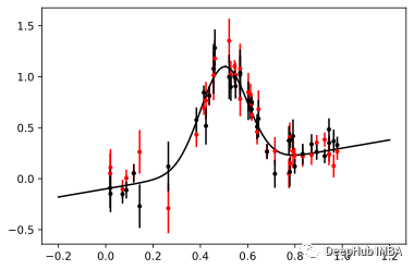
让我们来看看噪声仿真器的输出:
plt.errorbar(x, this_simulator(torch.tensor(theta)), yerr=y_err, fmt=".r", capsize=0)plt.errorbar(x, y, yerr=y_err, fmt=".k", capsize=0)plt.plot(x0, signal(theta, x0), "k", label="truth")
现在,我们使用 sbi 从这些模拟仿真中训练神经后验估计 (NPE)。
from sbi.inference.base import inferthis_simulator = lambda theta: simulator(theta, torch.tensor(x), torch.tensor(y_err))posterior = infer(this_simulator, prior, method='SNPE', num_simulations=10000)NPE使用条件归一化流来学习如何在给定一些数据的情况下生成后验分布:Running 10000 simulations.: 0%| | 0/10000 [00:00<?, ?it/s]Neural network successfully converged after 172 epochs.
在推理时,以实际数据 y 为条件简单地评估这个神经后验:
sbi_samples = posterior.sample((10000,), x=torch.tensor(y))sbi_samples = sbi_samples.detach().numpy()
可以看到速度非常快几乎不需要什么时间。
Drawing 10000 posterior samples: 0%| | 0/10000 [00:00, ?it/s]然后我们再次可视化后验样本:corner.corner(sbi_samples, labels=labels, truths=theta);
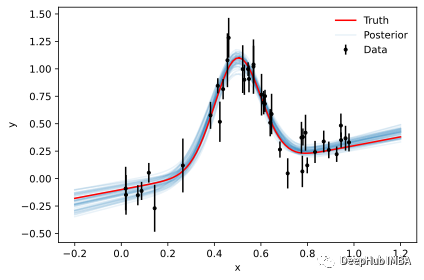
plot_results(x, y, y_err, samples=sbi_samples)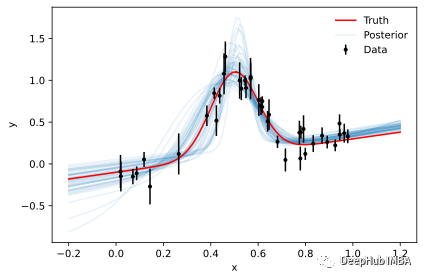
可以看到仿真SBI的的结果不如 MCMC 和 HMC 的结果。但是它们可以通过对更多模拟进行训练以及通过调整网络的架构来改进(虽然并不确定改完后就会有提高)。
但是我们可以看到即使在没有拟然性的情况下,SBI 也可以进行近似贝叶斯推理。
编辑:王菁
校对:林亦霖