
数学推导+纯Python实现机器学习算法15:GBDT
小白学视觉
共 10091字,需浏览 21分钟
· 2022-08-08
点击上方“小白学视觉”,选择加"星标"或“置顶”
重磅干货,第一时间送达

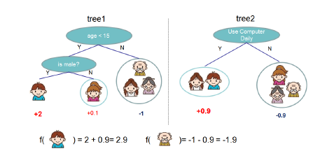
时隔大半年,机器学习算法推导系列终于有时间继续更新了。在之前的14讲中,笔者将监督模型中主要的单模型算法基本都过了一遍。预计在接下来的10讲中,笔者将努力更新完以GBDT代表的集成学习模型,以EM算法、CRF和隐马为代表的概率图模型以及以聚类降维为代表的无监督学习算法。


 (2) 对
(2) 对 有:
有:
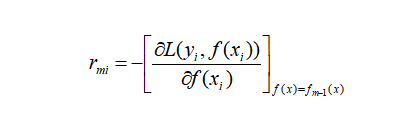
对每个样本
 ,计算负梯度,即残差

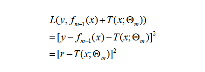
将上步得到的残差作为样本新的真实值,并将数据
 作为下棵树的训练数据,得到一颗新的回归树
 其对应的叶子节点区域为
 。其中
。其中 为回归树t的叶子节点的个数。
对叶子区域
 计算最佳拟合值

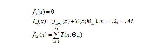
更新强学习器


class TreeNode():def __init__(self, feature_i=None, threshold=None,value=None, true_branch=None, false_branch=None):pass
class Tree(object):def __init__(self, min_samples_split=2, min_impurity=1e-7,max_depth=float("inf"), loss=None):self.root = None # Root node in dec. tree# Minimum n of samples to justify splitself.min_samples_split = min_samples_split# The minimum impurity to justify splitself.min_impurity = min_impurity# The maximum depth to grow the tree toself.max_depth = max_depth# Function to calculate impurity (classif.=>info gain, regr=>variance reduct.)# 切割树的方法,gini,方差等self._impurity_calculation = None# Function to determine prediction of y at leaf# 树节点取值的方法,分类树:选取出现最多次数的值,回归树:取所有值的平均值self._leaf_value_calculation = None# If y is one-hot encoded (multi-dim) or not (one-dim)self.one_dim = None# If Gradient Boostself.loss = lossdef fit(self, X, y, loss=None):""" Build decision tree """passdef _build_tree(self, X, y, current_depth=0):""" Recursive method which builds out the decision tree and splits X and respective ypassdef predict_value(self, x, tree=None):""" Do a recursive search down the tree and make a prediction of the data sample by thevalue of the leaf that we end up at """passdef predict(self, X):""" Classify samples one by one and return the set of labels """passdef print_tree(self, tree=None, indent=" "):pass
class RegressionTree(Tree):# 使用方差法进行树分割def _calculate_variance_reduction(self, y, y1, y2):var_tot = calculate_variance(y)var_1 = calculate_variance(y1)var_2 = calculate_variance(y2)frac_1 = len(y1) / len(y)frac_2 = len(y2) / len(y)# Calculate the variance reductionvariance_reduction = var_tot - (frac_1 * var_1 + frac_2 * var_2)return sum(variance_reduction)# 使用均值法取叶子结点值def _mean_of_y(self, y):value = np.mean(y, axis=0)return value if len(value) > 1 else value[0]# 回归树拟合def fit(self, X, y):self._impurity_calculation = self._calculate_variance_reductionself._leaf_value_calculation = self._mean_of_ysuper(RegressionTree, self).fit(X, y)
class Loss(object):def loss(self, y_true, y_pred):return NotImplementedError()def gradient(self, y, y_pred):raise NotImplementedError()def acc(self, y, y_pred):return 0class SquareLoss(Loss):def __init__(self): passdef loss(self, y, y_pred):return 0.5 * np.power((y - y_pred), 2)def gradient(self, y, y_pred):return -(y - y_pred)
class GBDT(object):def __init__(self, n_estimators, learning_rate, min_samples_split,min_impurity, max_depth, regression):# 基本参数self.n_estimators = n_estimatorsself.learning_rate = learning_rateself.min_samples_split = min_samples_splitself.min_impurity = min_impurityself.max_depth = max_depthself.regression = regressionself.loss = SquareLoss()if not self.regression:self.loss = SotfMaxLoss()# 分类问题也可以使用回归树,利用残差去学习概率self.estimators = []for i in range(self.n_estimators):self.estimators.append(RegressionTree(min_samples_split=self.min_samples_split,min_impurity=self.min_impurity,max_depth=self.max_depth))# 拟合方法def fit(self, X, y):# 让第一棵树去拟合模型self.estimators[0].fit(X, y)y_pred = self.estimators[0].predict(X)for i in range(1, self.n_estimators):gradient = self.loss.gradient(y, y_pred)self.estimators[i].fit(X, gradient)y_pred -= np.multiply(self.learning_rate, self.estimators[i].predict(X))# 预测方法def predict(self, X):y_pred = self.estimators[0].predict(X)for i in range(1, self.n_estimators):y_pred -= np.multiply(self.learning_rate, self.estimators[i].predict(X))if not self.regression:# Turn into probability distributiony_pred = np.exp(y_pred) / np.expand_dims(np.sum(np.exp(y_pred), axis=1), axis=1)# Set label to the value that maximizes probabilityy_pred = np.argmax(y_pred, axis=1)return y_pred
# regression treeclass GBDTRegressor(GBDT):def __init__(self, n_estimators=200, learning_rate=0.5, min_samples_split=2,min_var_red=1e-7, max_depth=4, debug=False):super(GBDTRegressor, self).__init__(n_estimators=n_estimators,learning_rate=learning_rate,min_samples_split=min_samples_split,min_impurity=min_var_red,max_depth=max_depth,regression=True)# classification treeclass GBDTClassifier(GBDT):def __init__(self, n_estimators=200, learning_rate=.5, min_samples_split=2,min_info_gain=1e-7, max_depth=2, debug=False):super(GBDTClassifier, self).__init__(n_estimators=n_estimators,learning_rate=learning_rate,min_samples_split=min_samples_split,min_impurity=min_info_gain,max_depth=max_depth,regression=False)def fit(self, X, y):y = to_categorical(y)super(GBDTClassifier, self).fit(X, y)
from sklearn import datasetsboston = datasets.load_boston()X, y = shuffle_data(boston.data, boston.target, seed=13)X = X.astype(np.float32)offset = int(X.shape[0] * 0.9)X_train, X_test, y_train, y_test = train_test_split(X, y, test_size=0.3)print(X_train.shape, y_train.shape, X_test.shape, y_test.shape)model = GBDTRegressor()model.fit(X_train, y_train)y_pred = model.predict(X_test)# Color mapcmap = plt.get_cmap('viridis')mse = mean_squared_error(y_test, y_pred)print ("Mean Squared Error:", mse)# Plot the resultsm1 = plt.scatter(range(X_test.shape[0]), y_test, color=cmap(0.5), s=10)m2 = plt.scatter(range(X_test.shape[0]), y_pred, color='black', s=10)plt.suptitle("Regression Tree")plt.title("MSE: %.2f" % mse, fontsize=10)plt.xlabel('sample')plt.ylabel('house price')plt.legend((m1, m2), ("Test data", "Prediction"), loc='lower right')plt.show();

好消息!
小白学视觉知识星球
开始面向外开放啦👇👇👇
下载1:OpenCV-Contrib扩展模块中文版教程 在「小白学视觉」公众号后台回复:扩展模块中文教程,即可下载全网第一份OpenCV扩展模块教程中文版,涵盖扩展模块安装、SFM算法、立体视觉、目标跟踪、生物视觉、超分辨率处理等二十多章内容。 下载2:Python视觉实战项目52讲 在「小白学视觉」公众号后台回复:Python视觉实战项目,即可下载包括图像分割、口罩检测、车道线检测、车辆计数、添加眼线、车牌识别、字符识别、情绪检测、文本内容提取、面部识别等31个视觉实战项目,助力快速学校计算机视觉。 下载3:OpenCV实战项目20讲 在「小白学视觉」公众号后台回复:OpenCV实战项目20讲,即可下载含有20个基于OpenCV实现20个实战项目,实现OpenCV学习进阶。 交流群
欢迎加入公众号读者群一起和同行交流,目前有SLAM、三维视觉、传感器、自动驾驶、计算摄影、检测、分割、识别、医学影像、GAN、算法竞赛等微信群(以后会逐渐细分),请扫描下面微信号加群,备注:”昵称+学校/公司+研究方向“,例如:”张三 + 上海交大 + 视觉SLAM“。请按照格式备注,否则不予通过。添加成功后会根据研究方向邀请进入相关微信群。请勿在群内发送广告,否则会请出群,谢谢理解~

评论
数学推导+纯Python实现机器学习算法22:EM算法
Python机器学习算法实现Author:louwillMachine Learning Lab 从本篇开始,整个机器学习系列还剩下最后三篇涉及导概率模型的文章,分别是EM算法、CRF条件随机场和HMM隐马尔科夫模型。本文主要讲解一下EM(Ex...
机器学习实验室
0
数学推导+纯Python实现机器学习算法19:CatBoost
Python机器学习算法实现Author:louwillMachine Learning Lab 本文介绍GBDT系列的最后一个强大的工程实现模型——CatBoost。CatBoost与XGBoost、LightGBM并称为GBDT框架下三大主流模型。CatBoost是俄罗斯搜索巨头...
机器学习实验室
0