本文将系统全面的介绍自动机器学习的其中一个常用框架: TPOT，一起研习如何在 Python 中将 TPOT 用于 AutoML 和 Scikit-Learn 机器学习算法。分类和回归小案例，以及一些用户手册的介绍。快来和小猴子一起研习吧！

如果你在机器学习建模期间花费数小时甚至数天时间来，一直尝试挑选最佳管道和参数的过程，那么我建议你仔细阅读本文。

自动机器学习 (AutoML) 是指需要极少人工参与的情况下自动发现性能良好的模型用于预测建模任务的技术。

本文核心内容：

• TPOT 是一个用于 AutoML 的开源库，具有 scikit-learn 数据准备和机器学习模型。
• 如何使用 TPOT 自动发现分类任务的最佳模型。
• 如何使用 TPOT 自动发现回归任务的最佳模型。

TPOT简介

Tree-based Pipeline Optimization Tool^[1], 基于树的管道优化工具，简称 TPOT，是一个用于在 Python 中执行 AutoML 的开源库。

TPOT 使用基于树的结构来表示预测建模问题的模型管道，包括数据准备和建模算法以及模型超参数。它利用流行的 Scikit-Learn 机器学习库进行数据转换和机器学习算法，并使用遗传编程随机全局搜索过程来有效地发现给定数据集的性能最佳的模型管道。

… an evolutionary algorithm called the Tree-based Pipeline Optimization Tool (TPOT) that automatically designs and optimizes machine learning pipelines.

... 一种称为基于树的管道优化工具 (TPOT) 的进化算法，可自动设计和优化机器学习管道。

然后执行优化过程以找到对给定数据集执行最佳的树结构。具体来说，一种遗传编程算法，旨在对表示为树的程序执行随机全局优化。

TPOT uses a version of genetic programming to automatically design and optimize a series of data transformations and machine learning models that attempt to maximize the classification accuracy for a given supervised learning data set.

TPOT 使用遗传编程的一个版本来自动设计和优化一系列数据转换和机器学习模型，这些模型试图最大限度地提高给定监督学习数据集的分类精度。

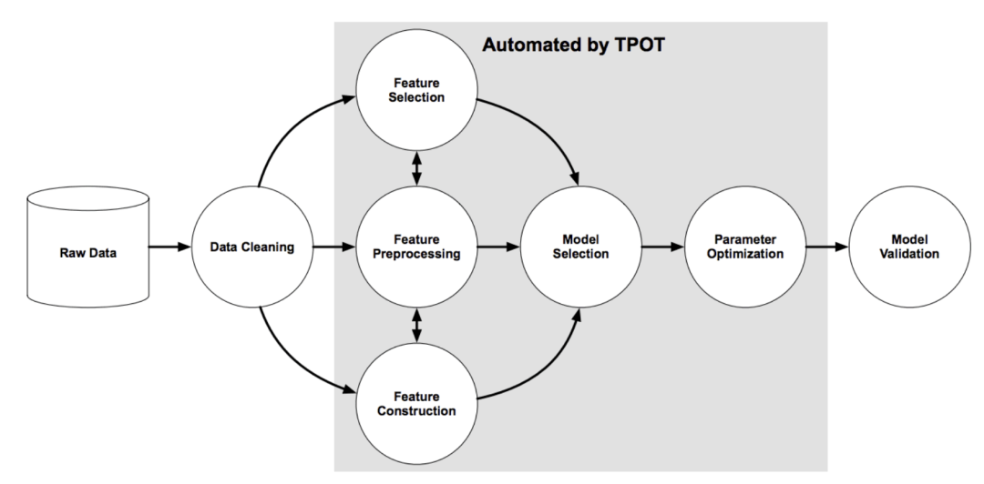
下图取自 TPOT 论文，展示了管道搜索所涉及的元素，包括数据清洗、特征选择、特征处理、特征构建、模型选择和超参数优化。

TPOT 将通过智能探索数千条可能的管道来为你的数据找到最佳管道，从而自动化机器学习中最繁琐的部分。

接下来我们一起看看如何安装和使用 TPOT 来找到一个有效的模型管道。

安装和使用 TPOT

第一步安装TPOT库

pip install tpot

安装后，导入库并打印版本号以确认它已成功安装：

# check tpot version
import tpot
print('tpot: %s' % tpot.__version__)

使用 TPOT 库很简单

需要创建TPOTRegressor 或 TPOTClassifier 类^[2]的实例，并做好配置后进行搜索，然后导出在数据集上找到的最佳性能的模型管道。

配置类涉及两个主要元素。

首先是如何评估模型，例如交叉验证方案和性能指标选择。建议使用选择的配置和要使用的性能指标明确指定交叉验证类。

例如要使用  neg_mean_absolute_error  作为回归度量，则选用RepeatedKFold^[3]用于回归交叉验证。

# 定义了评价步骤
cv = RepeatedKFold(n_splits=10, n_repeats=3, random_state=1)
# 定义搜索
model = TPOTRegressor(... scoring='neg_mean_absolute_error', cv=cv)

或者使用 accuracy 作为分类模型的评价指标，则选用RepeatedStratifiedKFold^[4] 用于分类交叉验证。

# 定义了评价步骤
cv = RepeatedStratifiedKFold(n_splits=10, n_repeats=3, random_state=1)
# 定义搜索
model = TPOTClassifier(... scoring='accuracy', cv=cv)

作为一种进化算法，涉及到较为复杂的配置的设置，例如种群规模、要运行的代数以及潜在的交叉和突变率。前者重要地控制着搜索的范围；如果你对进化搜索算法不熟悉，可以将后者保留设置为默认值。

例如，100 代和 5 或 10 代的适度种群规模是一个很好的起点。

# define 搜索
model = TPOTClassifier(generations=5, population_size=50, ...)

在搜索结束时，会找到性能最佳的管道。

此输出最佳模型的管道可以导出为py文件，后期可以将其复制并粘贴到你自己的项目中。

# 输出最佳模型
model.export('tpot_model.py')

TPOT 分类

这里使用 TPOT 来发现声纳数据集的最佳模型。

声纳数据集^[5]是一个标准的机器学习数据集，由 208 行数据和 60 个数字输入变量和一个具有两个类值的目标变量组成，例如二进制分类。

使用具有三个重复分层 10 折交叉验证的测试工具，朴素模型可以达到约 53% 的准确度。性能最佳的模型可以在相同的测试工具上实现大约 88% 的准确度。这达到了该数据集的预期性能界限。

该数据集涉及预测声纳返回是否指示岩石或矿井。

# summarize the sonar dataset
from pandas import read_csv
# load dataset
dataframe = read_csv(data, header=None)
# split into input and output elements
data = dataframe.values
X, y = data[:, :-1], data[:, -1]
print(X.shape, y.shape)

导入数据集并将其拆分为输入和输出数据集。可以看到有 60 个输入变量的 208 行数据。

首先，我们可以定义评估模型的方法，使用RepeatedStratifiedKFold交叉验证。

# 定义模型评估器
cv = RepeatedStratifiedKFold(n_splits=10, 
                             n_repeats=3, 
                             random_state=1)

将使用 50 个人口大小进行五折搜索，并设置 n_jobs = -1来使用系统上的所有核心。

# 定义搜索
model = TPOTClassifier(generations=5, 
                       population_size=50, cv=cv,
                       scoring='accuracy', verbosity=2,
                       random_state=1, n_jobs=-1)

最后，开始搜索并确保在运行结束时保存性能最佳的模型。

# 执行搜索
model.fit(X, y)
# 输出最佳模型
model.export('tpot_sonar_best_model.py')

这里可能需要运行几分钟，这里比较人性化的设置就是可以在命令行上看到一个进度条。

注意：你的结果可能会因算法或评估程序的随机性或数值精度的差异而有所不同。在现实案例中，可以多运行几次并比较平均结果。

将在此过程中将会输出报告性能最佳模型的准确性。

Generation 1 - Current best internal CV score: 0.8650793650793651
Generation 2 - Current best internal CV score: 0.8650793650793651
Generation 3 - Current best internal CV score: 0.8650793650793651
Generation 4 - Current best internal CV score: 0.8650793650793651
Generation 5 - Current best internal CV score: 0.8667460317460318

Best pipeline: GradientBoostingClassifier(GaussianNB(input_matrix),
learning_rate=0.1, max_depth=7, max_features=0.7000000000000001,
min_samples_leaf=15, min_samples_split=10, n_estimators=100, 
subsample=0.9000000000000001)

这里可以看到表现最好的管道达到了大约 86.6% 的平均准确率。这里接近该数据集上表现最好的模型了。

最后将性能最佳的管道保存到名为 “tpot_sonar_best_model.py ” 的文件中。

加载数据集和拟合管道的通用代码

# 在声纳数据集上拟合最终模型并做出预测的例子
from pandas import read_csv
from sklearn.preprocessing import LabelEncoder
from sklearn.model_selection import RepeatedStratifiedKFold
from sklearn.ensemble import GradientBoostingClassifier
from sklearn.naive_bayes import GaussianNB
from sklearn.pipeline import make_pipeline
from tpot.builtins import StackingEstimator
from tpot.export_utils import set_param_recursive
# 导入数据集
dataframe = read_csv(data, header=None)
# 拆分为输入变量和输出变量
data = dataframe.values
X, y = data[:, :-1], data[:, -1]
# 以尽量小的内存使用数据集
X = X.astype('float32')
y = LabelEncoder().fit_transform(y.astype('str'))
# 训练集上的交叉验证平均分数为: 0.8667
exported_pipeline = make_pipeline(
    StackingEstimator(estimator=GaussianNB()),
    GradientBoostingClassifier(learning_rate=0.1, max_depth=7, max_features=0.7000000000000001, min_samples_leaf=15, min_samples_split=10, n_estimators=100, subsample=0.9000000000000001)
)
# 修正了导出管道中所有步骤的随机状态
set_param_recursive(exported_pipeline.steps, 'random_state', 1)
# 训练模型
exported_pipeline.fit(X, y)
# 对新数据行进行预测
row = [0.0200,0.0371,0.0428,0.0207,0.0954,0.0986]
yhat = exported_pipeline.predict([row])
print('Predicted: %.3f' % yhat[0])

TPOT 回归

本节使用 TPOT 来发现汽车保险数据集的最佳模型。

汽车保险数据集^[6]是一个标准的机器学习数据集，由 63 行数据组成，一个数字输入变量和一个数字目标变量。

使用具有3 次重复的分层 10 折交叉验证的测试工具，朴素模型可以实现约 66 的平均绝对误差 (MAE)。性能最佳的模型可以在相同的测试工具上实现MAE约 28。这达到了该数据集的预期性能界限。

过程类似于分类。

加载数据集和拟合管道的通用代码

# 拟合最终模型并在保险数据集上做出预测的例子
from pandas import read_csv
from sklearn.model_selection import train_test_split
from sklearn.svm import LinearSVR
# 导入数据集
dataframe = read_csv(data, header=None)
# 拆分为输入变量和输出变量
data = dataframe.values
# 以尽量小的内存使用数据集
data = data.astype('float32')
X, y = data[:, :-1], data[:, -1]
# 训练集上的交叉验证平均分数为: -29.1476
exported_pipeline = LinearSVR(C=1.0, dual=False, epsilon=0.0001, loss="squared_epsilon_insensitive", tol=0.001)
# 修正了导出估计器中的随机状态
if hasattr(exported_pipeline, 'random_state'):
    setattr(exported_pipeline, 'random_state', 1)
# 模型训练
exported_pipeline.fit(X, y)
# 对新数据行进行预测
row = [108]
yhat = exported_pipeline.predict([row])
print('Predicted: %.3f' % yhat[0])

实战案例

Pima Indians Diabetes 数据集

这里有一个案例研究^[7]，使用 Pima Indians Diabetes 数据集预测 5 年内糖尿病的患病率。根据这项研究，作者指出在这个问题上达到的最大准确率为 77.47%。

在同一场景中进行自动化机器学习，看看它是如何使用 TPOT AutoML 工作的。

# import the AutoMLpackage after installing tpot.
import tpot
# 导入其他必要的包。
from pandas import read_csv
from sklearn.preprocessing import LabelEncoder
from sklearn.model_selection import StratifiedKFold
from tpot import TPOTClassifier
import os
# 导入数据
file_path = './pima-indians-diabetes.data.csv'
df = pd.read_csv(file_path,header=None) 
#可以用你自己的数据集.csv文件名替换
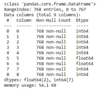
df.dtypes
df.info()

# 将数据帧的值拆分为输入和输出特征
data = df.values 
X, y = data[:, :-1], data[:, -1] 
print(X.shape, y.shape) 
#(768, 8 ) (768,) 
X = X.astype('float32') 
y = LabelEncoder().fit_transform(y.astype('str')) 
#模型评估定义，这里使用10倍StratifiedKFold 
cv = StratifiedKFold(n_splits=10) 
# 定义 TPOTClassifier 
model = TPOTClassifier(generations=5, population_size=50,
                       cv=cv, score='accuracy',
                       verbosity=2, random_state=1,
                       n_jobs=-1) 
# 执行最佳拟合搜索
model.fit(X , y) 
# 导出最佳模型
model.export('tpot_data.py')

我还用 cv=5 重复了上述实验。

# 模型评估定义，这里使用 5fold StratifiedKFold 
cv = StratifiedKFold(n_splits=5) 
# 定义 TPOTClassifier 
model = TPOTClassifier(generations=5, population_size=50,
                       cv=cv, score='accuracy', verbosity=2, 
                       random_state=1, n_jobs=-1) 
# 搜索最佳拟合
model.fit(X, y) 
# 导出最佳模型
model.export('tpot_data.py')

结果

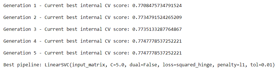
使用 10 折交叉验证时选择的最佳管道是：

LinearSVC(input_matrix, C=5.0, dual=False, 
          loss=squared_hinge,
          penalty=l1, tol=0.01)

# Accuracy: 77.47%

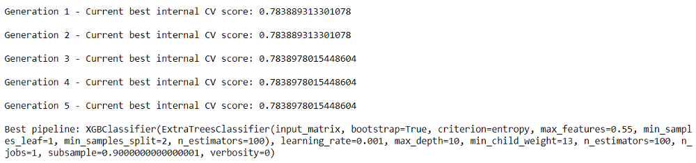
使用 5 折交叉验证时选择的最佳管道是：

XGBClassifier(ExtraTreesClassifier(input_matrix, bootstrap=True,
                                   criterion=entropy, max_features=0.55,
                                   min_samples_leaf=1, min_samples_split=2,
                                   n_estimators=100), 
              learning_rate=0.001, max_depth=10, 
              min_child_weight=13, n_estimators=100, 
              n_jobs=1, subsample=0.9000000000000001, 
              verbosity=0)

# Accuracy: 78.39%

TPOT和其他配置

为上述问题尝试了TPOT ，它仅使用默认配置。其实 AutoML TPOT 还有有许多内置配置。下面列出了这些变体：

• TPOT light： 如果你希望在管道中使用简单的运算符。此外，此配置确保这些运算符也可以快速执行。
• TPOT MDR： 如果你的问题属于生物信息学研究领域，并且此配置非常适合全基因组关联研究。
• TPOT sparse：如果你需要适合稀疏矩阵的配置。
• TPOT NN：如果你想利用默认 TPOT 的神经网络估计器。此外，这些估计器是用 PyTorch 编写的。
• TPOT cuML： 如果你的数据集大小为中型或大型，并且利用 GPU 加速的估计器在有限的配置上搜索最佳管道。

参考资料

精选文章