深度学习项目示例 | 手把手教你使用自编码器进行模糊图像修复-技术圈

来源：DeepHub IMBA
本文约2600字，建议阅读9分钟
本文教你如何应用深度学习处理模糊图像。

图像模糊是由相机或拍摄对象移动、对焦不准确或使用光圈配置不当导致的图像不清晰。为了获得更清晰的照片，我们可以使用相机镜头的首选焦点重新拍摄同一张照片，或者使用深度学习知识重现模糊的图像。由于我的专长不是摄影，只能选择使用深度学习技术对图像进行去模糊处理！

在开始这个项目之前，本文假定读者应该了解深度学习的基本概念，例如神经网络、CNN。还要稍微熟悉一下 Keras、Tensorflow 和 OpenCV。

有各种类型的模糊——运动模糊、高斯模糊、平均模糊等。但我们将专注于高斯模糊图像。在这种模糊类型中，像素权重是不相等的。模糊在中心处较高，在边缘处按照钟形曲线减少。

数据集

在开始使用代码之前，首先需要的是一个由 2 组图像组成的数据集——模糊图像和干净图像。目前可能没有现成的数据集可以使用，但是就像我们上面所说的，如果你有opencv的基础这个对于我们来说是非常个简单的，只要我们有原始图像，使用opencv就可以自己生成训练需要的数据集。

这里我的数据集大小约为 50 张图像（50 张干净图像和 50 张模糊图像），因为只是演示目的所以只选择了少量图像。

编写代码

已经准备好数据集，可以开始编写代码了。

依赖项


import numpy as npimport pandas as pdimport matplotlib.pyplot as plt
%matplotlib inlineimport randomimport cv2import osimport tensorflow as tffrom tqdm import tqdm

这里导入了 tqdm 库来帮助我创建进度条，这样可以知道运行代码需要多长时间。

导入数据


good_frames = '/content/drive/MyDrive/mini_clean'bad_frames = '/content/drive/MyDrive/mini_blur'

现在创建了2 个列表。我们将使用 keras 预处理库读取“.jpg”、“jpeg”或“.png”类型的图像，并转换为数组。这里图像尺寸为 128x128。


clean_frames = []for file in tqdm(sorted(os.listdir(good_frames))):if any(extension in file for extension in ['.jpg', 'jpeg', '.png']):  image = tf.keras.preprocessing.image.load_img(good_frames + '/' + file, target_size=(128,128))  image = tf.keras.preprocessing.image.img_to_array(image).astype('float32') / 255  clean_frames.append(image)
clean_frames = np.array(clean_frames)
blurry_frames = []for file in tqdm(sorted(os.listdir(bad_frames))):if any(extension in file for extension in ['.jpg', 'jpeg', '.png']):  image = tf.keras.preprocessing.image.load_img(bad_frames + '/' + file, target_size=(128,128))  image = tf.keras.preprocessing.image.img_to_array(image).astype('float32') / 255  blurry_frames.append(image)
blurry_frames = np.array(blurry_frames)

导入模型库


from keras.layers import Dense, Inputfrom keras.layers import Conv2D, Flattenfrom keras.layers import Reshape, Conv2DTransposefrom keras.models import Modelfrom keras.callbacks import ReduceLROnPlateau, ModelCheckpointfrom keras.utils.vis_utils import plot_modelfrom keras import backend as K
random.seed = 21np.random.seed = seed

将数据集拆分为训练集和测试集

现在我们按 80:20 的比例将数据集分成训练和测试集。

x = clean_frames;y = blurry_frames;
from sklearn.model_selection import train_test_splitx_train, x_test, y_train, y_test = train_test_split(x, y, test_size=0.2, random_state=42)

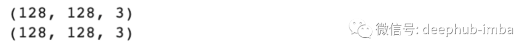
检查训练和测试数据集的形状。


print(x_train[0].shape)print(y_train[0].shape)


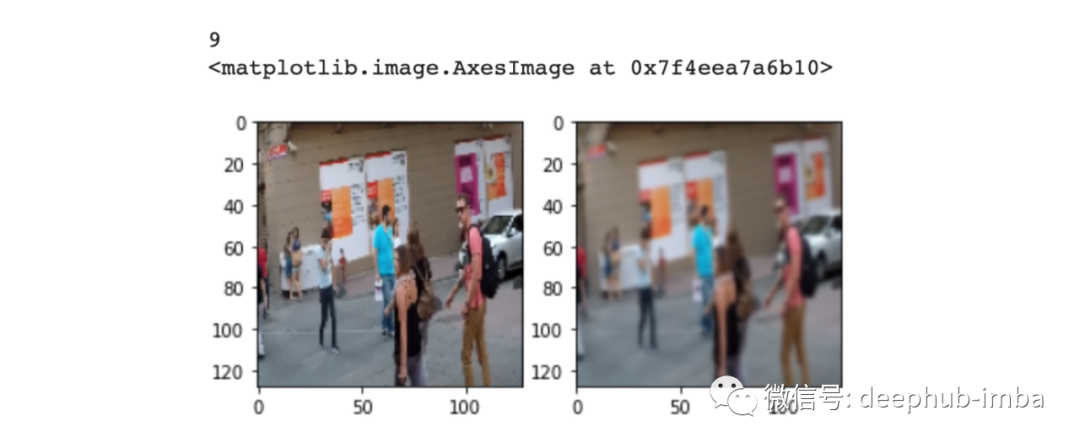
r = random.randint(0, len(clean_frames)-1)print(r)fig = plt.figure()fig.subplots_adjust(hspace=0.1, wspace=0.2)ax = fig.add_subplot(1, 2, 1)ax.imshow(clean_frames[r])ax = fig.add_subplot(1, 2, 2)ax.imshow(blurry_frames[r])

上面的代码可以查看来自训练和测试数据集的图像，例如：

下面初始化一些编写模型时需要用到的参数：


# Network Parametersinput_shape = (128, 128, 3)batch_size = 32kernel_size = 3latent_dim = 256
# Encoder/Decoder number of CNN layers and filters per layerlayer_filters = [64, 128, 256]

编码器模型

自编码器的结构我们以前的文章中已经详细介绍过多次了，这里就不详细说明了：


inputs = Input(shape = input_shape, name = 'encoder_input')x = inputs

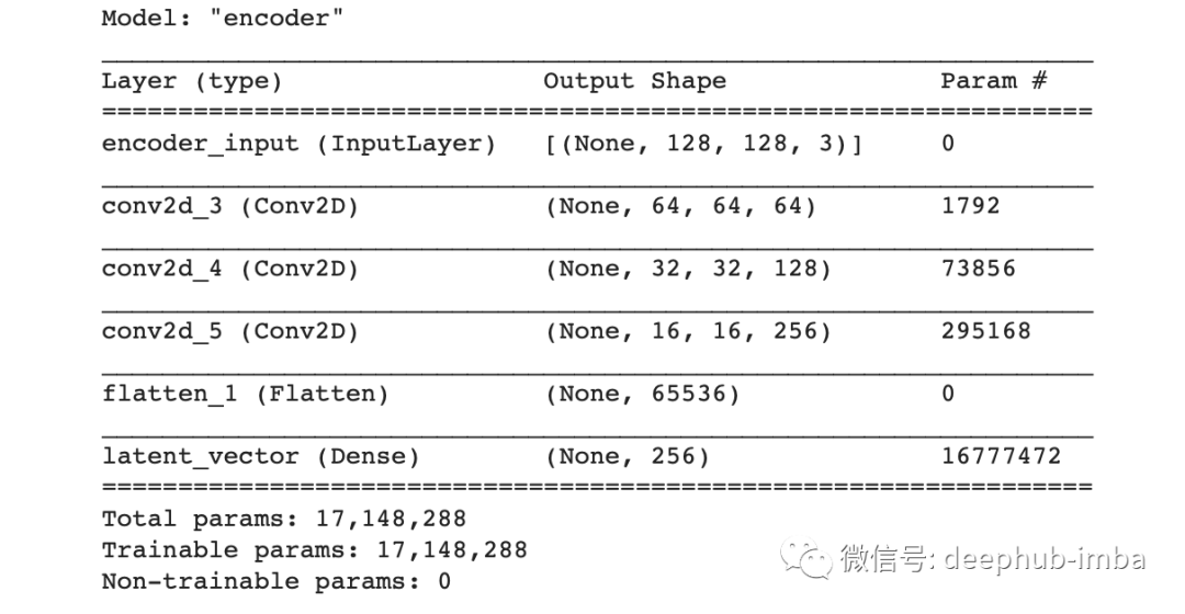
首先就是输入（图片的数组），获取输入后构建一个 Conv2D(64) - Conv2D(128) - Conv2D(256) 的简单的编码器，编码器将图片压缩为 (16, 16, 256) ，该数组将会是解码器的输入。


for filters in layer_filters:  x = Conv2D(filters=filters,              kernel_size=kernel_size,              strides=2,              activation='relu',              padding='same')(x)shape = K.int_shape(x)x = Flatten()(x)latent = Dense(latent_dim, name='latent_vector')(x)

这里的 K.int_shape()将张量转换为整数元组。

实例化编码器模型，如下：


encoder = Model(inputs, latent, name='encoder')encoder.summary()

解码器模型

解码器模型类似于编码器模型，但它进行相反的计算。解码器已将输入解码回 (128, 128, 3)。所以这里的将使用 Conv2DTranspose(256) - Conv2DTranspose(128) - Conv2DTranspose(64)。


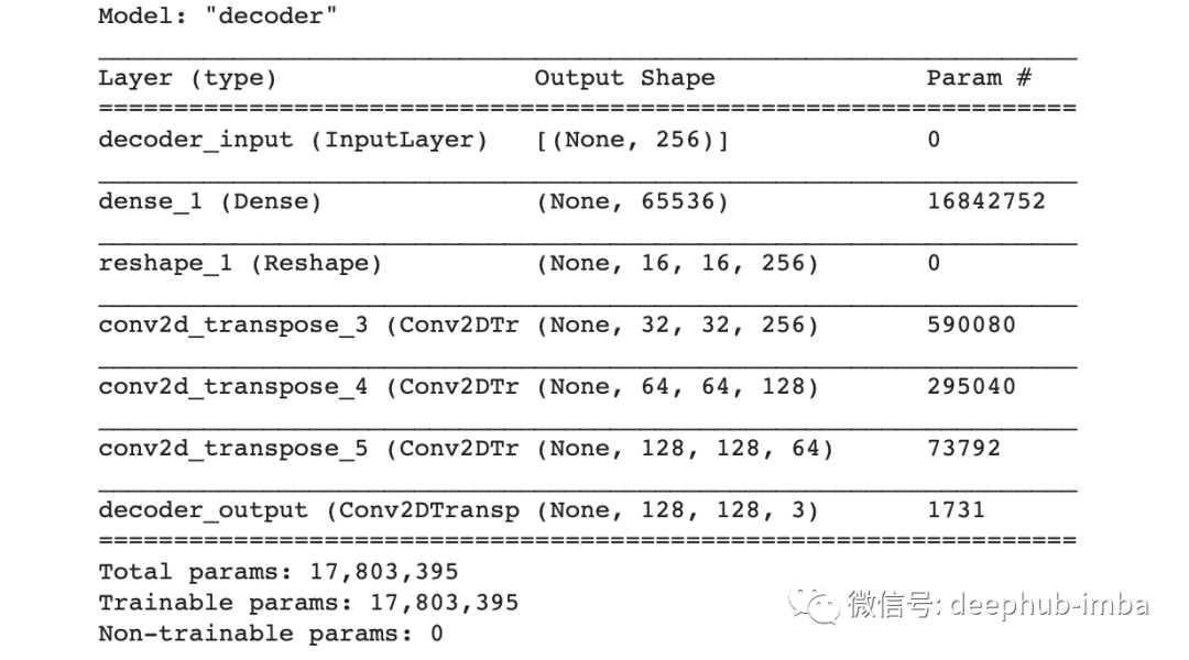
latent_inputs = Input(shape=(latent_dim,), name='decoder_input')x = Dense(shape[1]*shape[2]*shape[3])(latent_inputs)x = Reshape((shape[1], shape[2], shape[3]))(x)for filters in layer_filters[::-1]:  x = Conv2DTranspose(filters=filters,                      kernel_size=kernel_size,                      strides=2,                      activation='relu',                      padding='same')(x)
outputs = Conv2DTranspose(filters=3,                        kernel_size=kernel_size,                        activation='sigmoid',                        padding='same',                        name='decoder_output')(x)

解码器如下：


decoder = Model(latent_inputs, outputs, name='decoder')decoder.summary()

整合成自编码器

自编码器 = 编码器 + 解码器


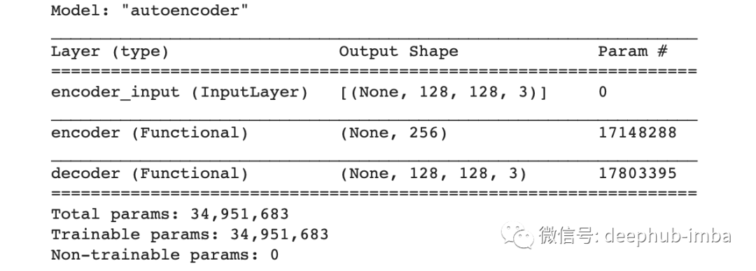
autoencoder = Model(inputs, decoder(encoder(inputs)), name='autoencoder')autoencoder.summary()

最后但是非常重要的是在训练我们的模型之前需要设置超参数。

autoencoder.compile(loss='mse', optimizer='adam',metrics=["acc"])

我选择损失函数为均方误差，优化器为adam，评估指标为准确率。然后还需要定义学习率调整的计划，这样可以在指标没有改进的情况下降低学习率：


lr_reducer = ReduceLROnPlateau(factor=np.sqrt(0.1),                              cooldown=0,                              patience=5,                              verbose=1,                              min_lr=0.5e-6)

学习率的调整需要在训练的每个轮次都调用：

callbacks = [lr_reducer]

训练模型


history = autoencoder.fit(blurry_frames,                    clean_frames,                    validation_data=(blurry_frames, clean_frames),                    epochs=100,                    batch_size=batch_size,                    callbacks=callbacks)

运行此代码后，可能需要大约 5-6 分钟甚至更长时间才能看到最终输出，因为我们设置了训练轮次为100：

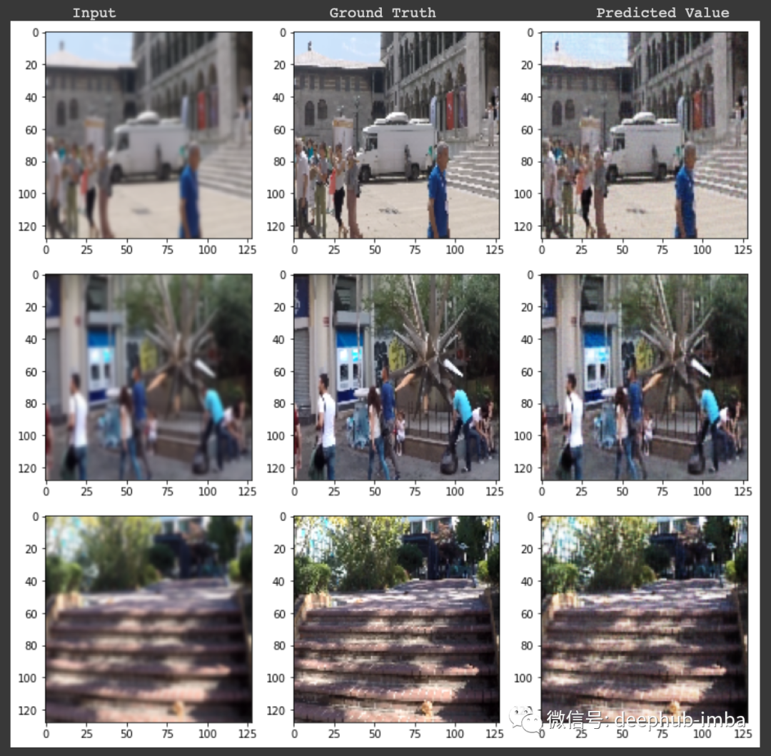
最后结果

现在已经成功训练了模型，让我们看看我们的模型的预测：


print("\n       Input                       Ground Truth                 Predicted Value")
for i in range(3):
  r = random.randint(0, len(clean_frames)-1)
  x, y = blurry_frames[r],clean_frames[r]  x_inp=x.reshape(1,128,128,3)  result = autoencoder.predict(x_inp)  result = result.reshape(128,128,3)
  fig = plt.figure(figsize=(12,10))  fig.subplots_adjust(hspace=0.1, wspace=0.2)
  ax = fig.add_subplot(1, 3, 1)  ax.imshow(x)
  ax = fig.add_subplot(1, 3, 2)  ax.imshow(y)
  ax = fig.add_subplot(1, 3, 3)  plt.imshow(result)

可以看到该模型在去模糊图像方面做得很好，并且几乎能够获得原始图像。因为我们只用了3层的卷积架构，所以如果我们使用更深的模型，还有一些超参数的调整应该会获得更好的结果。

为了查看训练的情况，可以绘制损失函数和准确率的图表，可以通过这些数据做出更好的决策。

损失的变化


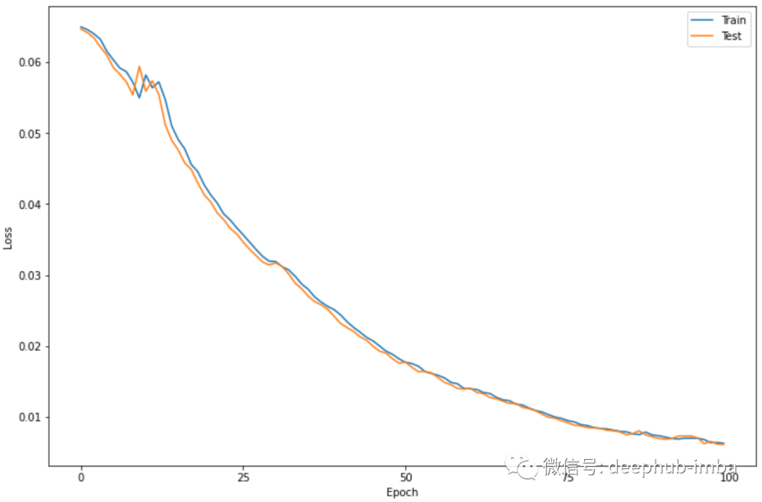
plt.figure(figsize=(12,8))plt.plot(history.history['loss'])plt.plot(history.history['val_loss'])plt.legend(['Train', 'Test'])plt.xlabel('Epoch')plt.ylabel('Loss')plt.xticks(np.arange(0, 101, 25))plt.show()

可以看到损失显著减少，然后从第 80 个 epoch 开始停滞不前。

准确率


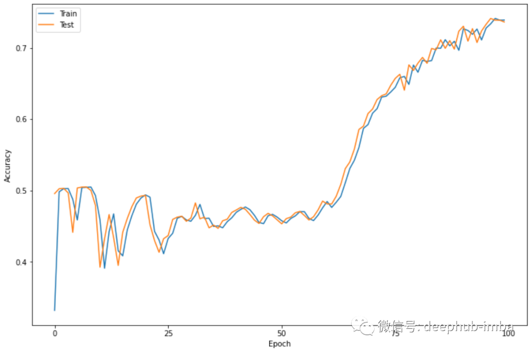
plt.figure(figsize=(12,8))plt.plot(history.history['acc'])plt.plot(history.history['val_acc'])plt.legend(['Train', 'Test'])plt.xlabel('Epoch')plt.ylabel('Accuracy')plt.xticks(np.arange(0, 101, 25))plt.show()