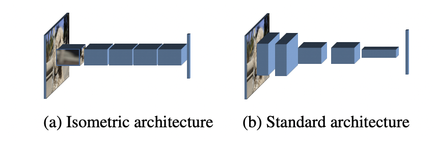
CNN迎来了新的变革：isotropic architecture

前段时间，一篇匿名论文Patches Are All You Need? 火了，这篇文章提出用基于卷积的block来替换ViT中的transformer block，这样就变成了基于patch的卷积网络ConvMixer，它和ViT模型一样都属于同质架构（isotropic architecture）：模型主体是由相同的blocks重复串联而成。一旦block固定，基于同质架构的模型只需要用特征大小（即patch embedding的维度）和网络深度（即blocks数量）两个参数定义。其实谷歌在提出ViT之后，在后续的工作MLP-Mixer中提出了用基于2个MLP的block来替换ViT中的transformer block，MetaAI同期也提出了训练更高效的版本ResMLP，它们都和ViT一样属于同质架构，区别就在于block不一样。虽然从网络设计上来看基于同质架构的模型更简单，但是主流的CNN模型往往不是同质架构，而是一种金字塔架构（pyramidal architecture），对比如下所示，这种金字塔架构包含几个不同的stage，各个stage之间是一个下采样操作比如stride=2的max pooling或者conv。CNN常用的金字塔架构好处在于下采样可以较快地增大感受野，而且下采样也降低了特征图大小，从而计算上更高效。而ConvMixer打破了这种经典的金字塔架构设计，不过这并不是最早的工作，比如谷歌在2019年就提出了Isotropic MobileNetv3，但这个工作并未受到较大的关注，另外MetaAI在ResMLP论文中也探讨了用卷积来替换MLP。而MeatAI在最新的论文Augmenting Convolutional networks with attention-based aggregation中设计了一种性能更优的PatchConvNet，相比ConvMixer，PatchConvNet在速度和准确度上都更好，而且PatchConvNet也在密集任务如检测和分割上表现优异。本文将简单地介绍这些相关的工作以及它们的区别和联系。

MLP-Mixer和ResMLP

继ViT之后，谷歌又提出了只包含MLP架构的MLP-Mixer，如下图所示。相比ViT，MLP-Mixer也是先经过patch embedding layer得到patch tokens，然后送入N个相同的blocks，区别就在于这里的block不再是transformer block，而是包含两个MLP的Mixer Layer。这里的第一个MLP用于实现token mixing（对特征矩阵转置），这个就相当于transformer block中的self-attention模块，用于建立tokens间的信息交互，而第二个MLP用于实现channel mixing，这个和transformer block中FFP模块完全一致，用于建立每个token的channels间的信息交互。MLP-Mixer和ViT一样，都是全局建模，而且也都是同质架构。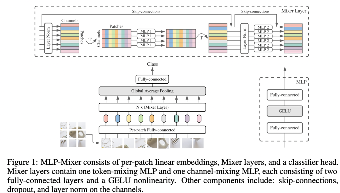虽然谷歌在论文中通过实验证明了MLP-Mixer可以达到和ViT类似的效果，但是比较依赖大规模数据的预训练。相较之下，MeatAI同期的工作ResMLP只使用ImageNet-1K数据集，和DeiT一样，它是通过采用heavy的数据增强策略来消除对大规模训练数据的依赖。在架构上，ResMLP基本和MLP-Mixer一样，一个区别是ResMLP block中用于tokens间交互的模块只用了一个fc层，而不是包含2个fc层的MLP，另外ResMLP采用了一种更简单的norm layer来替换LayerNorm。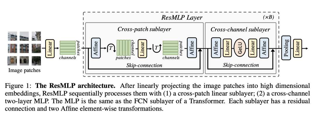ResMLP的PyTorch代码实现如下所示，作为一种同质架构，整体的代码实现是比较简洁的。

# No norm layer                                                                                                                             
class Affine(nn.Module):
    def __init__(self, dim):
        super().__init__()
        self.alpha = nn.Parameter(torch.ones(dim))
        self.beta = nn.Parameter(torch.zeros(dim))
    def forward(self, x): 
        return self.alpha * x + self.beta

# MLP on channels
class Mlp(nn.Module):
    def __init__(self, dim):
        super().__init__()
        self.fc1 = nn.Linear(dim, 4 * dim)
        self.act = nn.GELU()
        self.fc2 = nn.Linear(4 * dim, dim)
    def forward(self, x): 
        x = self.fc1(x)
        x = self.act(x)
        x = self.fc2(x)
        return x

# ResMLP blocks: a linear between patches + a MLP to process them independently
class ResMLP_BLocks(nn.Module):
    def __init__(self, nb_patches ,dim, layerscale_init):
        super().__init__()
        self.affine_1 = Affine(dim)
        self.affine_2 = Affine(dim)
        self.linear_patches = nn.Linear(nb_patches, nb_patches) #Linear layer on patches
        self.mlp_channels = Mlp(dim) #MLP on channels
        self.layerscale_1 = nn.Parameter(layerscale_init * torch.ones((dim))) #LayerScale
        self.layerscale_2 = nn.Parameter(layerscale_init * torch.ones((dim))) # parameters
    def forward(self, x): 
        res_1 = self.linear_patches(self.affine_1(x).transpose(1,2)).transpose(1,2))
        x = x + self.layerscale_1 * res_1
        res_2 = self.mlp_channels(self.affine_2(x))
        x = x + self.layerscale_2 * res_2
        return x

# ResMLP model: Stacking the full network
class ResMLP_models(nn.Module):
    def __init__(self, dim, depth, nb_patches, layerscale_init, num_classes):
        super().__init__()
        self.patch_projector = Patch_projector()
        self.blocks = nn.ModuleList([
        ResMLP_BLocks(nb_patches ,dim, layerscale_init)
        for i in range(depth)])
        self.affine = Affine(dim)
        self.linear_classifier = nn.Linear(dim, num_classes)
    def forward(self, x):
        B, C, H, W = x.shape
        x = self.patch_projector(x)
        for blk in self.blocks:
            x = blk(x)
        x = self.affine(x)
        x = x.mean(dim=1).reshape(B,-1) #average pooling
        return self.linear_classifier(x)

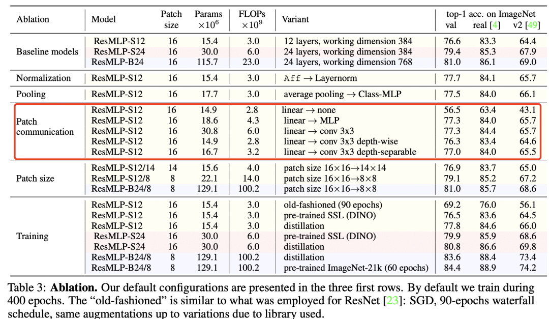
既然MLP都有效，那么一个问题是如果采用基于卷积的block，这种同质架构还有效吗？其实，谷歌在MLP-Mixer论文中也讨论了MLP-Mixer和CNN的联系：用于channel mixing的MLP可以用1x1卷积实现，而token mixing MLP可以用一个kernel size为image size的depth-wise conv来实现（这里各个channel的参数是共享的）。因而MLP-Mixer其实也可以看成一种特殊的CNN架构。虽然1x1卷积是比较常见的，但是kernel size等于image size的卷积并不是一种常规的卷积（虽然对特征矩阵转置后，token-mixing MLP实际上也可以1x1卷积实现，但这个也不是CNN的常规操作），那么问题是能否用常规的卷积如3x3卷积来实现token mixing MLP，这个问题可以在ResMLP论文中找到答案。ResMLP只用了一个FC层来实现token mixing，其weights可视化如下图所示，可以看到在前面的layers其表现出局部性，虽然理论上token mixing是可以实现全局感受野的，但是它实际的行为却和卷积比较类似，这提示可以用卷积来替换FC。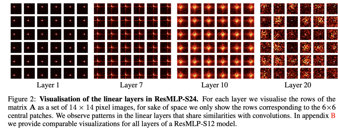论文尝试了用3x3 conv，3x3 depth-wise conv和3x3 depth-separable conv来替代这个FC层，发现模型效果并没有太多变化，比如采用轻量级的3x3 depth-wise conv，其参数量和FLOPs都降低了，但是模型效果只下降了0.3（76.3 vs 76.6）。这样替换之后，网络就变成了一个纯粹基于卷积的同质架构，这与之前常用的金字塔架构相区别：

This suggests that convolutions on low-resolution feature maps at all layers is an interesting alternative to the common pyramidal design of convnets, where early layers operate at higher resolution and smaller feature dimension.

这里要讨论的一点是，无论是self-attention还是MLP，它们在理论上都可以实现全局建模，但是卷积没有这种优势，因为它只能实现局部建模，不过通过堆积大量的卷积层，感受野最终也可以达到全局，而且卷积的这种inductive bias对CV任务也有天然优势。而在架构方面，self-attention和卷积都能处理变输入，而MLP（token mixing）只能处理固定输入。

ConvMixer

ConvMixer这篇工作motivation是来自于谷歌的MLP-Mixer，其设计思路是：用kernel size比较大的conv实现token mixing，而用pointwise conv（即1x1 conv）来实现channel mixing。ConvMixer的整体架构如下所示：

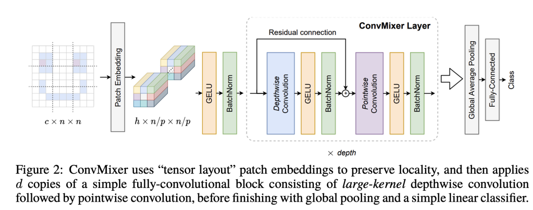这种设计和ResMLP的conv版本区别主要有两点：一是ConvMixer采用kernel size较大（eg. 9x9）的depth-wise conv来实现token mixing；二是ConvMixer只用了一个1x1 conv来实现channel mixing，而ResMLP是用一个MLP，这等价于2个1x1 conv。ConvMixer采用较大的kernel size是想实现较大的感受野，但其实ResMLP却已经证明3x3 conv也是能够实现好的性能。ConvMixer的代码实现如下所示：

class Residual(nn.Module):
    def __init__(self, fn):
        super().__init__()
        self.fn = fn

    def forward(self, x):
        return self.fn(x) + x

def ConvMixer(dim, depth, kernel_size=9, patch_size=7, n_classes=1000):
    return nn.Sequential(
        nn.Conv2d(3, dim, kernel_size=patch_size, stride=patch_size),
        nn.GELU(),
        nn.BatchNorm2d(dim),
        *[nn.Sequential(
                Residual(nn.Sequential(
                    nn.Conv2d(dim, dim, kernel_size, groups=dim, padding="same"),
                    nn.GELU(),
                    nn.BatchNorm2d(dim)
                )),
                nn.Conv2d(dim, dim, kernel_size=1),
                nn.GELU(),
                nn.BatchNorm2d(dim)
        ) for i in range(depth)],
        nn.AdaptiveAvgPool2d((1,1)),
        nn.Flatten(),
        nn.Linear(dim, n_classes)
    )

虽然ConvMixer在同样的参数量下效果可以达到或者超过ResNet，ResMLP和DeiT，但是由于使用较大的kernel size，而且ConvMixer也采用了较小的patch size（7x7，这样特征图较大），这导致其计算量较大，速度较慢。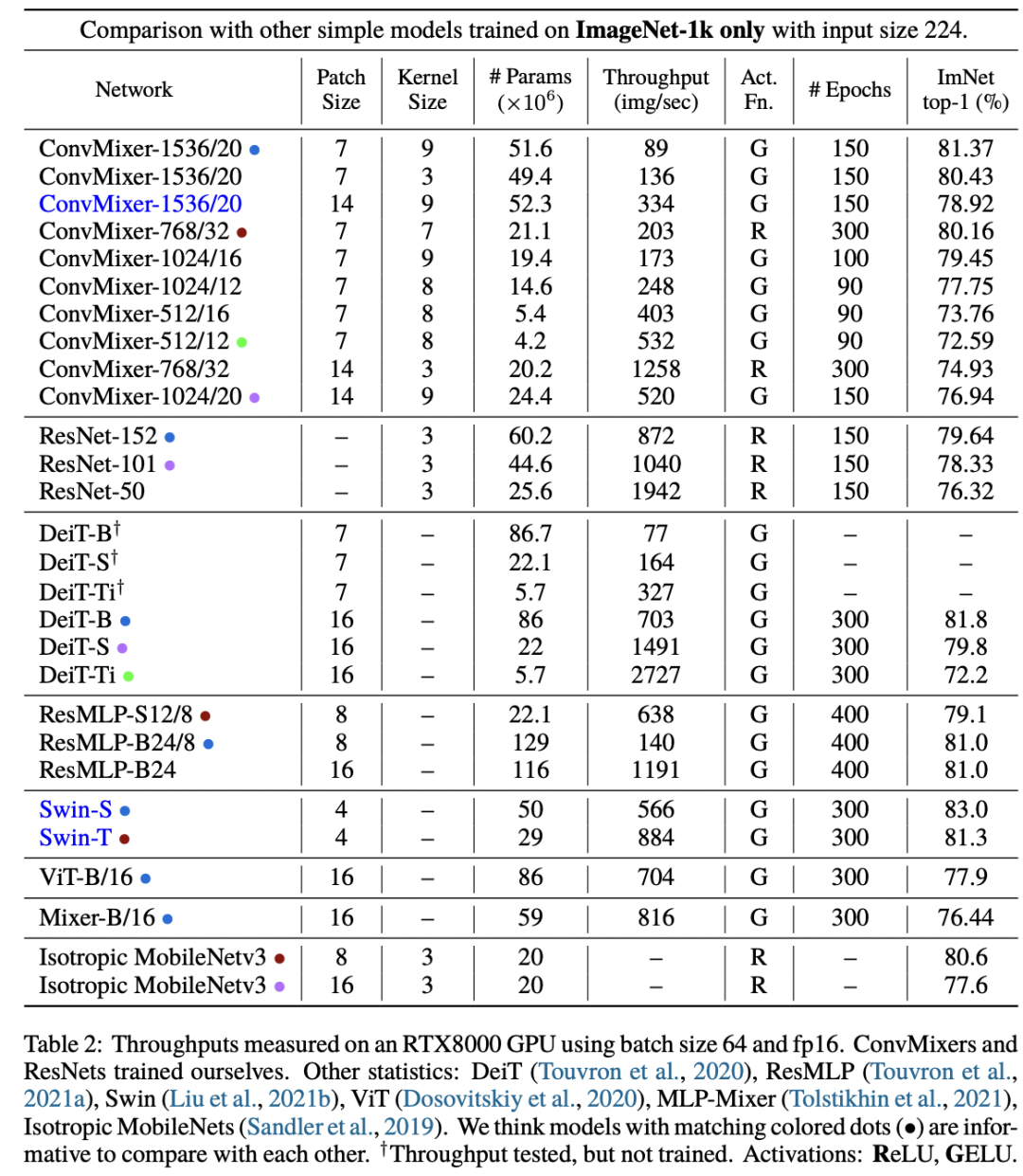ConvMixer和ViT，MLP-Mixer的一个共同点就是它们都是基于patch的模型，所以论文说：patches are all you need，但其实它们更大的一个相似点是：它们都属于同质架构。

PatchConvNet

PatchConvNet是MetaAI在最近的论文Augmenting Convolutional networks with attention-based aggregation提出的，虽然这个论文的主题是用attention-based aggregation（即attention-based pooling）来替换CNN中常用的global average pooling从而增强模型性能，但论文采用的是一种基于patch的同质CNN架构。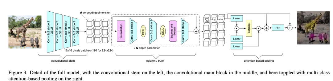相比ConvMixer，PatchConvNet采用了convolutional stem来提取patch embedding，而不是采用一个简单linear projection，这个问题在论文Early Convolutions Help Transformers See Better被详细地研究过：ViT原来地linear projection等价于一个stride=p且kernel_size=p的conv，如果把它转换成几个堆叠的stride=2的3*3 conv，无论是在模型效果上，还是在训练稳定性以及收敛速度都更好。具体地，PatchConvNet采用的patch size为16x16，这样把它转换为4个stride=2的3x3卷积，代码实现如下所示（这里每经过一个conv，channels也double，最终达到patch embedding的维度大小）：

def conv3x3(in_planes, out_planes, stride=1):
    """3x3 convolution with padding"""
    return torch.nn.Sequential(
        nn.Conv2d(
            in_planes, out_planes, kernel_size=3, stride=stride, padding=1, bias=False
        ),
    )

class ConvStem(nn.Module):
    """ Image to Patch Embedding
    """
    def __init__(self, img_size=224, patch_size=16, in_chans=3, embed_dim=768):
        super().__init__()
        img_size = to_2tuple(img_size)
        patch_size = to_2tuple(patch_size)
        num_patches = (img_size[1] // patch_size[1]) * (img_size[0] // patch_size[0])
        self.img_size = img_size
        self.patch_size = patch_size
        self.num_patches = num_patches

        self.proj = torch.nn.Sequential(
            conv3x3(3, embed_dim // 8, 2),
            nn.GELU(),
            conv3x3(embed_dim // 8, embed_dim // 4, 2),
            nn.GELU(),
            conv3x3(embed_dim // 4, embed_dim // 2, 2),
            nn.GELU(),
            conv3x3(embed_dim // 2, embed_dim, 2),
        )

    def forward(self, x, padding_size=None):
        B, C, H, W = x.shape
        x = self.proj(x).flatten(2).transpose(1, 2)
        return x

在block设计方面，PatchConvNet采用了基于SE的residual block（1x1 conv -> 3x3 depth-wise conv -> SE -> 1x1 conv），这个是CNN中最常用的结构。注意这里采用了pre-norm，只在block的开始采用norm layer，可以使用BatchNorm或者LayerNorm，虽然BatchNorm能比LayerNorm实现更好的性能，但BatchNorm比较依赖batch size，所以论文默认采用LayerNorm。具体的代码实现如下（这里采用了CaiT中提出的LayerScale）：

class Conv_blocks_se(nn.Module):
    def __init__(self, dim):
        super().__init__()
        
        self.qkv_pos = nn.Sequential(
            nn.Conv2d(dim, dim, kernel_size = 1),
            nn.GELU(),
            nn.Conv2d(dim, dim, groups = dim, kernel_size = 3, padding = 1, stride = 1, bias = True),
            nn.GELU(),
            SqueezeExcite(dim, rd_ratio=0.25),
            nn.Conv2d(dim, dim, kernel_size=1),
        )

    def forward(self, x):
        B, N, C = x.shape
        H = W = int(N**0.5)
        x = x.transpose(-1,-2)
        x = x.reshape(B,C,H,W)
        x = self.qkv_pos(x)
        x = x.reshape(B,C,N)
        x = x.transpose(-1,-2)
        return x

    
class Layer_scale_init_Block(nn.Module):

    def __init__(self, dim,drop_path=0., act_layer=nn.GELU, norm_layer=nn.LayerNorm,
                 Attention_block=Conv_blocks_se, init_values=1e-4):
        super().__init__()
        self.norm1 = norm_layer(dim)
        self.attn = Attention_block(dim)
        self.drop_path = DropPath(drop_path) if drop_path > 0. else nn.Identity()
        self.gamma_1 = nn.Parameter(init_values * torch.ones((dim)),requires_grad=True)

    def forward(self, x):
        return x + self.drop_path(self.gamma_1 * self.attn(self.norm1(x)))

最后一点是PatchConvNet采用了attention-based pooling而不是global average pooling，后者是CNN最常采用的，即简单地取对所有patches的特征求平均，而attention-based pooling是基于attention的加权平均。具体地，增加一个可训练的class token，先对所有的patches做attention得到加权平均，然后加上class token送入一个FFN。具体的代码实现如下所示：

class Learned_Aggregation_Layer(nn.Module):
    def __init__(self, dim, num_heads=1, qkv_bias=False, qk_scale=None, attn_drop=0., proj_drop=0.):
        super().__init__()
        self.num_heads = num_heads
        head_dim = dim // num_heads
        
        self.scale = qk_scale or head_dim ** -0.5

        self.q = nn.Linear(dim, dim, bias=qkv_bias)
        self.k = nn.Linear(dim, dim, bias=qkv_bias)
        self.v = nn.Linear(dim, dim, bias=qkv_bias)
        self.attn_drop = nn.Dropout(attn_drop)
        self.proj = nn.Linear(dim, dim)
        self.proj_drop = nn.Dropout(proj_drop)


    
    def forward(self, x ):
        
        B, N, C = x.shape
        q = self.q(x[:,0]).unsqueeze(1).reshape(B, 1, self.num_heads, C // self.num_heads).permute(0, 2, 1, 3)
        k = self.k(x).reshape(B, N, self.num_heads, C // self.num_heads).permute(0, 2, 1, 3)

        q = q * self.scale
        v = self.v(x).reshape(B, N, self.num_heads, C // self.num_heads).permute(0, 2, 1, 3)
        
        
        attn = (q @ k.transpose(-2, -1))
        attn = attn.softmax(dim=-1)
        attn = self.attn_drop(attn)

        x_cls = (attn @ v).transpose(1, 2).reshape(B, 1, C)
        x_cls = self.proj(x_cls)
        x_cls = self.proj_drop(x_cls)
        
        
        return x_cls
    
 class Layer_scale_init_Block_only_token(nn.Module):

    def __init__(self, dim, num_heads, mlp_ratio=4., qkv_bias=False, qk_scale=None, drop=0., attn_drop=0.,
                 drop_path=0., act_layer=nn.GELU, norm_layer=nn.LayerNorm, Attention_block = Learned_Aggregation_Layer, Mlp_block=Mlp,
                 init_values=1e-4):
        super().__init__()
        self.norm1 = norm_layer(dim)
        self.attn = Attention_block(
            dim, num_heads=num_heads, qkv_bias=qkv_bias, qk_scale=qk_scale, attn_drop=attn_drop, proj_drop=drop)
        # NOTE: drop path for stochastic depth, we shall see if this is better than dropout here
        self.drop_path = DropPath(drop_path) if drop_path > 0. else nn.Identity()
        self.norm2 = norm_layer(dim)
        mlp_hidden_dim = int(dim * mlp_ratio)
        self.mlp = Mlp_block(in_features=dim, hidden_features=mlp_hidden_dim, act_layer=act_layer, drop=drop)
        self.gamma_1 = nn.Parameter(init_values * torch.ones((dim)),requires_grad=True)
        self.gamma_2 = nn.Parameter(init_values * torch.ones((dim)),requires_grad=True)

    def forward(self, x, x_cls):
        u = torch.cat((x_cls,x),dim=1)
        x_cls = x_cls + self.drop_path(self.gamma_1 * self.attn(self.norm1(u)))
        x_cls = x_cls + self.drop_path(self.gamma_2 * self.mlp(self.norm2(x_cls)))
        return 

从实现上来看，其实attention-based pooling就是一个简化的transformer block，这里在做attention时query只有class token，而且attention head设置为1，这个设计也是在CaiT中提出的。attention-based pooling的好处是直接用attention map就可以可视化分类模型的决策，而CNN往往需要一些复杂的方法如CAM来做可视化，而ViT由于涉及不同的layers和heads也需要特殊处理attention map。这里默认采用一个class token，也可以每个类都定义一个单独的class token，这样可以得到每个类的attention map，不过这样计算量也变大了。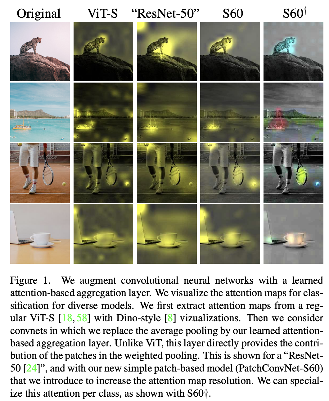PatchConvNet由于是同质架构，只需要两个参数就可以定义：特征维度大小和网络深度（blocks数量）。论文共设置3种不同的特征大小：384，768和1024，分别用S，B和L表示，比如S60模型就表示特征大小是384，而blocks数量为60，这个模型在参数量和FLOPs上和ResNet50相当。PatchConvNet由于是同质架构，所以在推理阶段，其使用的memory量是恒定的（不考虑前后处理，即conv stem和attention-based pooling），另外PatchConvNet的一个特性它的peak memory是较低的，而且和图像大小基本上是线性关系，如下图所示，而ViT这样的模型其peak memory与图像大小的平方成正比，当输入图像增大时，peak memory增长较快，这对于输入较大的分割和检测任务是非常不友好的。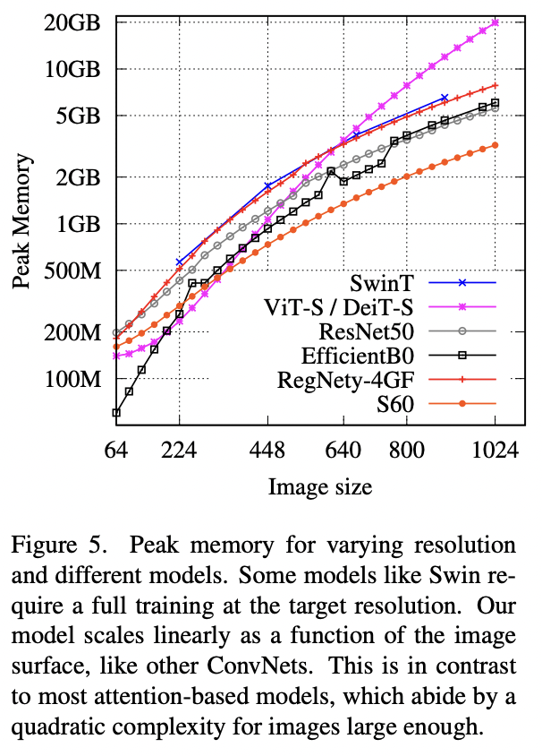PatchConvNet在ImageNet1K数据集上表现如下表所示，其在准确度和计算量上均表现较好。比如S60模型，其FLOPs和throughout和Swin-T类似，但效果比Swin-T更好，而且peak memory远低于Swin-T（不过PatchConvNet训练的epoch是400，而Swin训练的epoch是300，两者的训练策略基本一致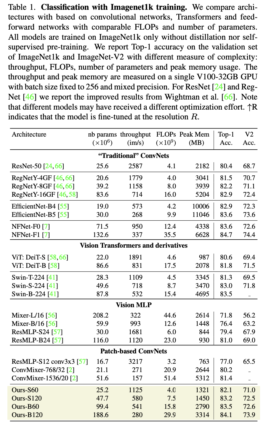）。PatchConvNet在分割和检测任务上也表现优异，如下表所示。由于分割和检测往往需要多尺度的输入，而PatchConvNet只输出1/16大小的特征，这里采用XciT的解决方案，即对PatchConvNet的中间输出通过上采样（stride=2的2x2反卷积）或者下采样（stride=2的2x2 max pooling）来得到不同尺度的特征。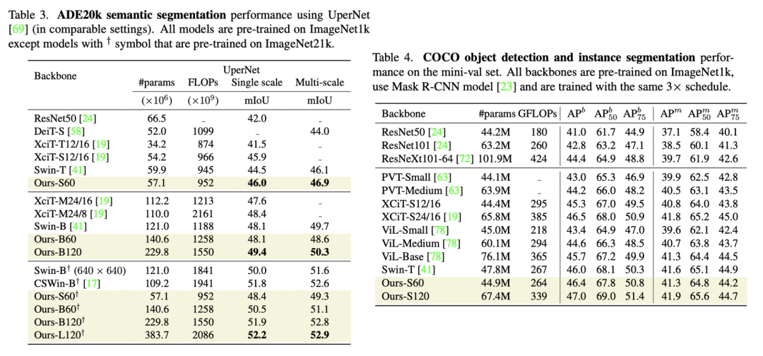PatchConvNet的消融实验如下所示，这里是基于S60模型，可以看到对性能影响最大的是采用conv stem，如果换成linear projection，性能会下降2个点；而将LayerNorm换成BatchNorm，大约可以提升0.3个点；而如果采用简单的global average pooling，性能只掉了0.2个点，这说明attention-based pooling其实对性能影响较小，如果去掉attention-based pooling，那么PatchConvNet就真正成为一个完全的CNN了。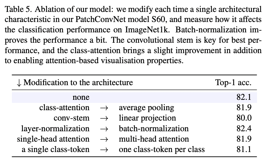相比ConvMixer，PatchConvNet在设计上做了很多的优化比如conv stem和SE，而且PatchConvNet网络是更深，比如S60其主体就包含了180个conv layers，这也远超ResNet50和ConvMixer的层数，或许采用3x3卷积加上更深的网络能够带来弥补感受野的不足。

小结

本文简单介绍了最近几个基于同质架构的CNN模型，相比常用的金字塔架构，这应该算是一种改变，而且MetaAI设计的PatchConvNet也取得了较好的效果，并且可以应用在分割和检测任务上。这也让我们重新思考是否有必要采用金字塔架构，因为同质架构设计上更简单，未来金字塔架构是否被完全取代，这值得探讨。

参考

• ResMLP: Feedforward networks for image classification with data-efficient training
• MLP-Mixer: An all-MLP Architecture for Vision
• Patches Are All You Need?
• https://github.com/facebookresearch/deit
• Augmenting Convolutional networks with attention-based aggregation