动手学geopandas地理数据分析

公众号后台回复关键字："源码"，获取本文全部代码！

一，GeoPandas总体介绍

geopandas 是pandas在地理数据处理领域的扩展包，主要基于Pandas(普通数据处理), shapely(地理数据分析),fiona(地理数据读取),matplotlib(地理数据可视化)等构建而成。

其核心数据结构是GeoSeries和GeoDataFrame。

其中GeoSeries是pandas中的Series的一个子类，GeoDataFrame是Pandas中的DataFrame的一个子类。

GeoSeries是一列有几何形状(Point,LineString,Polygon,MultiLineString,……)等构成的数据列。

GeoDataFrame由多列Series或者GeoSeries组成，其中至少需要有一列为GeoSeries。

并且需要设置其中的一列GeoSeries为当前活跃状态的GeoSeries，默认的地理数据分析操作都是对活跃状态的GeoSeries进行的。

geopandas 的以下功能非常常用：

• 1，文件读写

• 2，空间查询

• 3，坐标转换

• 4，空间join

• 5，地理数据可视化

#安装geopandas
!pip install -i https://pypi.tuna.tsinghua.edu.cn/simple geopandas 

import numpy as np 
import pandas as pd 
import shapely 
import geopandas as gpd 
from shapely import wkt 
from shapely import geometry as geo 
from matplotlib import pyplot as plt 
import rtree 

二，GeoSeries常用操作

1， 创建GeoSeries

gsr_points = gpd.GeoSeries([geo.Point(0.0,0.0),geo.Point(1.0,1.0),geo.Point(2.0,3.0)]) 
print(gsr_points)

0    POINT (0.00000 0.00000)
1    POINT (1.00000 1.00000)
2    POINT (2.00000 3.00000)
dtype: geometry

2，常用属性方法

#注：一般来说GeoSeries和空间相关的属性和方法对于GeoDataFrame也是适用的
gsr_polygons = gsr_points.buffer(0.5)
print("area:\n",gsr_polygons.area)
print("length:\n",gsr_polygons.length)
print("total_bounds:\n",gsr_polygons.total_bounds)

print("bounds:\n",gsr_polygons.bounds)
print("centroid:\n",gsr_polygons.centroid)
print("distances:\n",gsr_polygons.distance(geo.Point(0,0)))

area:
 0    0.784137
1    0.784137
2    0.784137
dtype: float64
length:
 0    3.140331
1    3.140331
2    3.140331
dtype: float64
total_bounds:
 [-0.5 -0.5  2.5  3.5]
bounds:
    minx  miny  maxx  maxy
0  -0.5  -0.5   0.5   0.5
1   0.5   0.5   1.5   1.5
2   1.5   2.5   2.5   3.5
centroid:
 0    POINT (-0.00000 -0.00000)
1      POINT (1.00000 1.00000)
2      POINT (2.00000 3.00000)
dtype: geometry
distances:
 0    0.000000
1    0.914214
2    3.105552
dtype: float64

ax = gsr_polygons.plot(figsize = (8,10),cmap = "tab10") 
gsr_points.plot(color = "red",ax = ax)

三，GeoDataFrame常用操作

1，文件读写

#可以直接读geojson和shp等空间文件，也可以读含有geometry字段的csv文件
dfraw = gpd.read_file(gpd.datasets.get_path('naturalearth_lowres'))

#保存成geojson
dfraw.to_file("dfcountries.geojson",driver = "GeoJSON")

#读取geojson
dfload = gpd.read_file("dfcountries.geojson",bbox = [-180,-80,180,80]) #可以用bbox或mask过滤范围


#保存成csv，继承pandas接口
dfload.to_csv("dfcountries.csv",index = False,sep = "\t")


#pandas读取csv,再转成GeoDataFrame
dfcsv = pd.read_csv("dfcountries.csv",sep = "\t")
dfcsv["geometry"] = dfcsv["geometry"].apply(wkt.loads)
df = gpd.GeoDataFrame(dfcsv,geometry = "geometry")

2，空间查询

#空间查询可以建立rtree快速找到某个范围内的对象，GeoSeries也具有该功能
sindex = df.sindex 

#可以调用intersection方法用一个bbox（可以来自geom.bounds）来进行查询
selected_ids = sindex.intersection(np.array([-120,-45,120,45]))

#可以调用query方法用一个geometry来进行查询, 查询关系可以用 predicate指定('intersect','contains','within'等)

query_ids = sindex.query(geo.Polygon.from_bounds(-120,-45,120,45))
print(df.loc[query_ids,:].shape) 

#查看predicate可用的取值参数
print(sindex.valid_query_predicates)

(139, 6)
{'within', 'touches', 'crosses', 'intersects', 'overlaps', None, 'contains'}

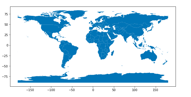
3，坐标转换

# 设置坐标系
dfwgs = df.set_crs("EPSG:4326") #df.set_crs(epsg=4326)
print(dfwgs.crs)  

dfwgs.plot()

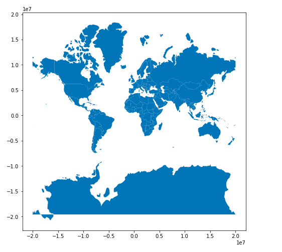
#转换成墨卡托
dfmercator = dfwgs.to_crs("EPSG:3395")
print(dfmercator.crs)
dfmercator.plot() 

4， 空间join

#空间join实际上是利用空间索引实现的。
#两个GeoDataFrame通过几何之间的‘intersects’,‘contains’,'crosses'等关系可以建立配对关系，从而确定join逻辑。
#join的类型可以是left,right或者inner 

dfcountries = gpd.read_file(gpd.datasets.get_path('naturalearth_lowres'))
dfcities = gpd.read_file(gpd.datasets.get_path('naturalearth_cities'))
dfjoin = gpd.sjoin(dfcities,dfcountries,op= 'intersects',how = "left")

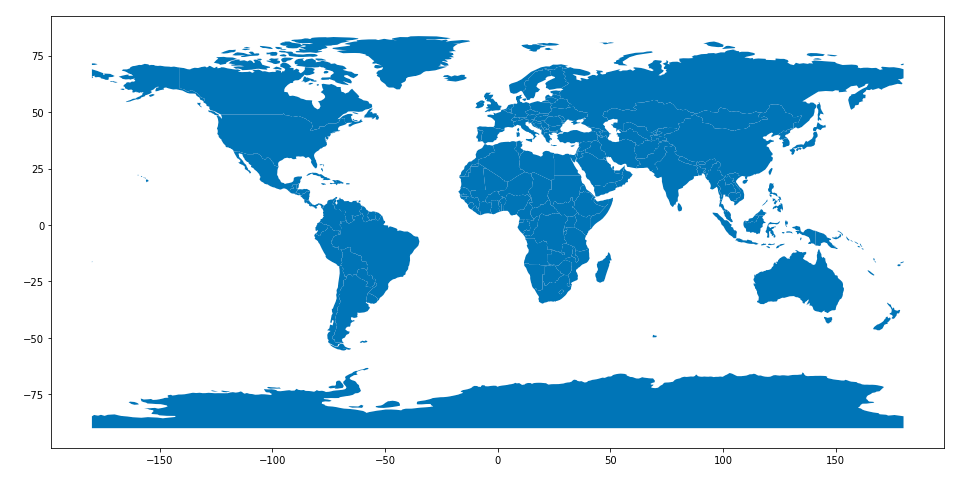
5，可视化

#利用GeoDataFrame可以像DataFrame那样方便地调用plot函数进行可视化操作。
#和DataFrame的plot函数相比，GeoDataFrame的plot函数的kind参数在"line","bar"等基础上增加了"geo”类型的绘图类别。

%matplotlib inline 
%config InlineBackend.figure_format = 'png'
from matplotlib import pyplot as plt 

df = gpd.read_file(gpd.datasets.get_path('naturalearth_lowres'))

#绘制简单形状
df.plot(kind="geo",figsize = (16,13)) 

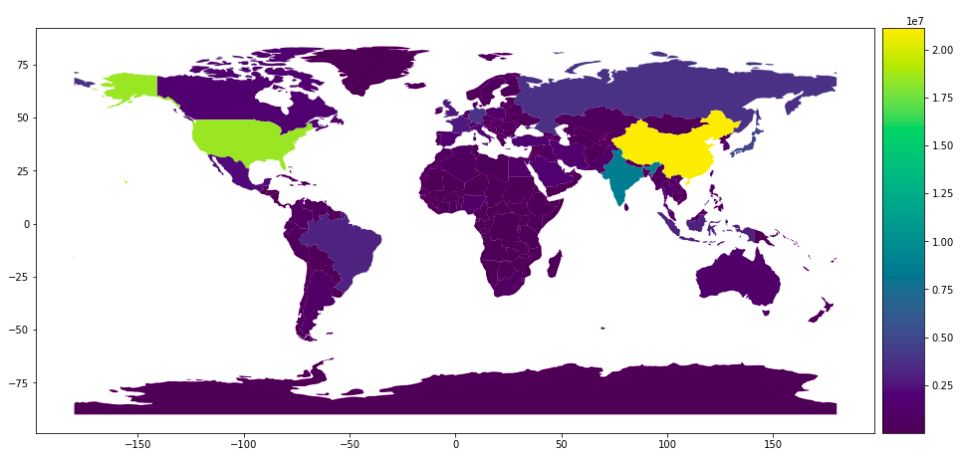
#绘制属性
%matplotlib inline 
%config InlineBackend.figure_format = 'png'

from mpl_toolkits.axes_grid1 import make_axes_locatable
fig, ax = plt.subplots(1, 1,figsize = (16,13))
divider = make_axes_locatable(ax)
cax = divider.append_axes("right", size="5%", pad=0.1)

df = gpd.read_file(gpd.datasets.get_path('naturalearth_lowres'))
df.plot(kind="geo",column = "gdp_md_est",legend=True,ax = ax,cax = cax  ) 

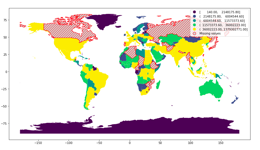
#属性图考虑缺失值
df = gpd.read_file(gpd.datasets.get_path('naturalearth_lowres'))
df.loc[np.random.choice(df.index, 20), 'pop_est'] = np.nan 
df.plot(column="pop_est",figsize=(15, 10),scheme = 'Quantiles',legend=True,
        missing_kwds={"color": "lightgrey","edgecolor": "red","hatch": "///","label": "Missing values"} ) 

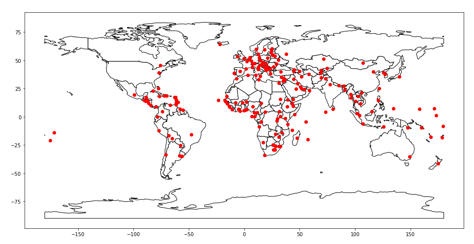
#多图叠加
dfcoutries = gpd.read_file(gpd.datasets.get_path('naturalearth_lowres'))
ax = dfcoutries.plot(kind="geo",figsize = (16,13),color='white', edgecolor='black') 
dfcities = gpd.read_file(gpd.datasets.get_path('naturalearth_cities'))
dfcities.plot(color = "red",ax = ax)