 大邓和他的Python


01. 引言
本期推文回归学术图表的绘制教程,本次的推文也是在查看SCI论文时发现,图表简单明了且使用较多,接下来我们通过构建虚拟数据进行符合出版的多类别散点图绘制。
02. 数据构建及可视化绘制
我们构建6组虚拟数据进行绘制,具体如下:
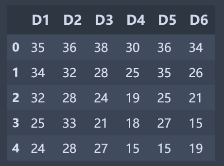
绘图代码具体如下:
#开始绘图import numpy as npimport pandas as pdimport matplotlib.pyplot as pltfrom matplotlib.pyplot import MultipleLocatorplt.rcParams['font.family'] = "Times New Roman"x = np.arange(0,len(scatter),1)y1 = scatter.D1.valuesy2 = scatter.D2.valuesy3 = scatter.D3.valuesy4 = scatter.D4.valuesy5 = scatter.D5.valuesy6 = scatter.D6.valuesfig,ax = plt.subplots(figsize=(4.5,3),dpi=300)scatter_01 = ax.plot(x,y1,marker='s',c='k',lw=.5,markerfacecolor='dimgray',markeredgecolor='dimgray',label='D1')scatter_02 = ax.plot(x,y2,marker='s',c='k',ls='--',lw=.5,markerfacecolor='white',markeredgewidth=.4,markeredgecolor='k',label='D2')scatter_03 = ax.plot(x,y3,marker='o',c='k',lw=.8,ls=':',markerfacecolor='dimgray',markeredgecolor='dimgray',label='D3')scatter_04 = ax.plot(x,y4,marker='o',c='k',lw=.5,markerfacecolor='white',markeredgewidth=.4,markeredgecolor='k',label='D4')scatter_05 = ax.plot(x,y5,marker='^',c='k',lw=.5,ls='-.',markerfacecolor='k',markeredgecolor='k',label='D5')scatter_06 = ax.plot(x,y6,marker='^',c='k',ls='--',lw=.5,markerfacecolor='white',markeredgewidth=.4,markeredgecolor='k',label='D6')#修改次刻度yminorLocator = MultipleLocator(2.5) #将此y轴次刻度标签设置为0.1的倍数ax.yaxis.set_minor_locator(yminorLocator)ax.tick_params(which='major',direction='out',length=4,width=.5)ax.tick_params(which='minor',direction='out',length=2,width=.5)ax.set_ylim(bottom=10,top=45)for spine in ['top','bottom','left','right']:ax.spines[spine].set_linewidth(.5)ax.legend(frameon=False,ncol=3,loc='upper center',fontsize=8.5)text_font = {'size':'13','weight':'bold','color':'black'}ax.text(.03,.91,"(a)",transform = ax.transAxes,fontdict=text_font,zorder=4)ax.text(.87,.04,'\nVisualization by DataCharm',transform = ax.transAxes,ha='center', va='center',fontsize = 4,color='black',fontweight='bold',family='Roboto Mono')plt.savefig(r'F:\DataCharm\SCI paper plots\sci_scatter.png',width=4.5,height=3,dpi=900,bbox_inches='tight')plt.show()
知识点:
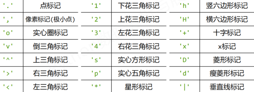
(1)ax.plot()函数marker的具体设置,本期推文,我们分别设置's' 矩形,'o'圆形,'^' 上三角形。其他类型如下:
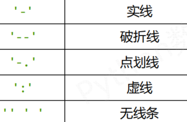
(2)ax.plot()函数linestyle(ls)连接线的类型,matplotlib提供的类别如下:
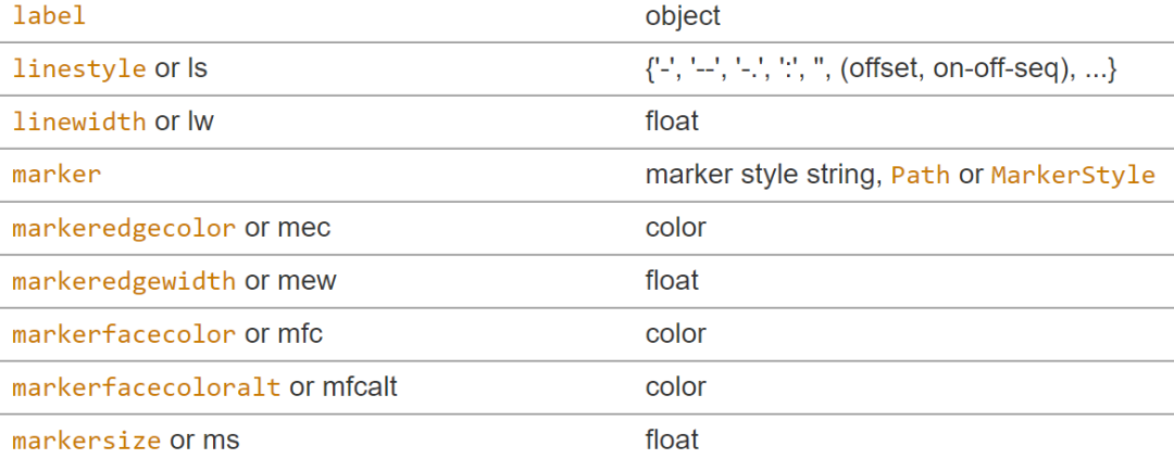
下面列举ax.plot()其他主要参数如下:
(3) 副刻度设置:ax.yaxis.set_minor_locato()
(4) 轴脊(spines)宽度设置:
for spine in ['top','bottom','left','right']:ax.spines[spine].set_linewidth(.5)
其他详细内容可以参考官网
得到的图形如下:

03. 总结
本期推文回归学术图表绘制教程:多类别散点图。涉及连接线、颜色、刻度等属性参数的设置,教程相对简单,希望能够帮到大家。
近期文章
Python网络爬虫与文本数据分析 rpy2库 | 在jupyter中调用R语言代码 tidytext | 耳目一新的R-style文本分析库 reticulate包 | 在Rmarkdown中调用Python代码 plydata库 | 数据操作管道操作符>> plotnine: Python版的ggplot2作图库 七夕礼物 | 全网最火的钉子绕线图制作教程 读完本文你就了解什么是文本分析 文本分析在经管领域中的应用概述 综述:文本分析在市场营销研究中的应用 plotnine: Python版的ggplot2作图库 小案例: Pandas的apply方法 stylecloud:简洁易用的词云库 用Python绘制近20年地方财政收入变迁史视频 Wow~70G上市公司定期报告数据集 漂亮~pandas可以无缝衔接Bokeh YelpDaset: 酒店管理类数据集10+G